Canonical correlation
At our seminar earlier this year I looked at the validity of assumptions underpinning some stochastic projection models for mortality. I looked at the assumption of parameter independence in forecasting, and examined whether this assumption was borne out by the data. It transpires that the assumption of independence is a workable assumption for some models, but not for others. This has important consequences in a Solvency II context — an internal model must be shown to have assumptions grounded in fact.
To illustrate, we contrast two models which share a number of features. First, the Lee-Carter model:
and second the age-period-cohort (APC) model:
Forecasting in these models depends on an assumption of independence as follows: in the Lee-Carter model we fix the α and β parameters at their estimated values and forecast κ independently of these values; in the APC model we fix the α parameter at its estimated value and then forecast κ and γ independently of each other and of α. In the rest of this posting we examine the validity of these independence assumptions.
Both these models need constraints on the parameters to fix unique estimates. In the Lee-Carter model we use the following constraints:
while for the Age-Period-Cohort model we use the following:
where wc is the cohort weight, i.e. the number of times cohort c appears in the data.
Parameter estimates are usually correlated in most statistical models, and the situation here is complicated by the constraints. We can use the concept of canonical correlation to measure the strength of the association between the different estimates. We won't go into the details — the interested reader can find more here — but suffice to say that a canonical correlation varies from 0 (no correlation between parameters) to 1 (perfect correlation between parameters). We will denote the canonical correlation between two vector variables x and y as r(x, y). The assumption of independence between x and y means that r(x, y) should be zero.
First, the Lee-Carter model, where we find that r(α, κ) = 0.21. This isn't ideal — it clearly isn't zero. However, the APC model is even worse, as r(α,κ) = 0.44, r(α, γ) = 0.56 and r(κ, γ) = 0.66. Should we worry about these correlations? Figure 1 shows some plots of bivariate normal variables with different degrees of correlation:
Figure 1. Samples of size 1000 from bivariate normal distributions with correlations 0.01, 0.21, 0.66 and 1.0 respectively. Source: own simulations.
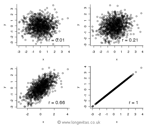
The top two panels in Figure 1 suggest that we can be relatively relaxed about the correlation between parameters in the Lee-Carter model. Visually, there is not too much of a difference between zero and 0.21. However, the same cannot be said for the APC model — the bottom left panel shows that a canonical correlation of 0.66 is quite different from zero.
Where does this leave us? There are real cohort effects in many data sets, both in the UK and other countries. Models with cohort effects will therefore fit the past data better, and it is natural to try and incorporate these cohort effects in forecasting methods. However, the measured cohort effects do not exist independently of either the age effect (r(α, γ) = 0.56) or the period effect (r(κ, γ) = 0.66). Forecasting with the APC model is therefore more complicated than the independence assumption implies. In contrast, the Lee-Carter model doesn't fit as well as the APC model but its forecasting assumptions are more soundly based.
Add new comment