The age pattern of mortality

Heligman and Pollard published a famous paper in 1980 with the title "The age pattern of mortality". In their paper they proposed an additive, three-component model of mortality:

\[q_x/p_x = f_I(x) + f_S(x) + f_A(x)\]

where \(f_I(x)\) describes infant and child mortality, \(f_S(x)\) is underlying mortality (senescence) for the whole of life and \(f_A(x)\) is the "accident hump'". Here \(q_x\) is the probability of dying within one year for a person aged \(x\) exactly, \(p_x = 1 - q_x\). These three components reflect almost universal patterns in human mortality and, on the log scale, Heligman and Pollard's components are:

1. \(\log f_I(x) = A(x+B)^C\), i.e. a power of \(x\),
2. \(\log f_S(x) = G + Hx\), i.e. a straight line in \(x\), and
3. \(\log f_A(x) = D - E(\log x - \log F)^2\), i.e. quadratic in \(\log x\).

This blog, in homage to Heligman and Pollard, has the same title as their paper. Our purpose is to introduce an alternative approach to modelling these three components which has recently been proposed by Camarda, Eilers and Gampe (CEG). They propose replacing the specific parametric functions of Heligman and Pollard by general smooth functions. We set up some notation. Let \(\boldsymbol{d} = (d_1, \ldots, d_n)^\prime\) be the observed numbers of deaths at ages \(x_1, \ldots, x_n\), and \(\boldsymbol{e} = (e_1, \ldots, e_n)^\prime\) be the corresponding central exposures. Let \(\boldsymbol{D}\) be the random variable corresponding to \(\boldsymbol{d}\) and \(\mbox{E} [\boldsymbol{D}] = \boldsymbol{\mu} = (\mu_1, \ldots, \mu_n)^\prime\). The random part of the CEG model is \(D_i \sim \mbox{Poisson}(\mu_i)\) and its systematic part is:

\[\boldsymbol{\mu}/\boldsymbol{e} = \boldsymbol{\gamma_I} + \boldsymbol{\gamma_S} + \boldsymbol{\gamma_A}\]

where \(\boldsymbol{\gamma_I}=(\gamma_{I,1},\ldots,\gamma_{I,n})^\prime\), \(\boldsymbol{\gamma_S}=(\gamma_{S,1},\ldots,\gamma_{S,n})^\prime\) and \(\boldsymbol{\gamma_A}=(\gamma_{A,1},\ldots,\gamma_{A,n})^\prime\) are the three components corresponding to \(f_I(x)\), \(f_S(x)\) and \(f_A(x)\) respectively. CEG now assume that each of the components is smooth in \(x\) and, corresponding to (1), (2) and (3) above, we have:

\[\log \boldsymbol{\gamma_I} = \boldsymbol{B_I\alpha_I},\; \log \boldsymbol{\gamma_S} = \boldsymbol{B_S\alpha_S}, \;\log \boldsymbol{\gamma_A} = \boldsymbol{B_A\alpha_A},\]

where \(\boldsymbol{B_I}\), \(\boldsymbol{B_S}\) and \(\boldsymbol{B_A}\) are regression matrices of cubic \(B\)-splines, and \(\boldsymbol{\alpha_I}\), \(\boldsymbol{\alpha_S}\) and \(\boldsymbol{\alpha_A}\) are the corresponding regression coefficients. Penalties on the coefficients \(\boldsymbol{\alpha_I}\), \(\boldsymbol{\alpha_S}\) and \(\boldsymbol{\alpha_A}\) are used in the usual \(P\)-spline way (Eilers & Marx, 1996) to bring about appropriate smoothness.

The Heligman-Pollard model is not easy to fit. For example Jones (2005) reports that "the HP model is a beast to fit. The parameters are highly correlated and this causes tremendous identifiability problems'". It appears that we have the same problem here, only worse. The three bases overlap and there is nothing so far that enables the three components to be identified. So here comes the clever bit! CEG use strong penalties (in addition to the smoothness penalties in the previous paragraph) to force

• \(\boldsymbol{\gamma_I}\), infant and child mortality, to be monotonic decreasing,
• \(\boldsymbol{\gamma_S}\), senescent mortality, to be monotonic increasing, and
• \(\boldsymbol{\gamma_A}\), accident mortality, to be log-concave.

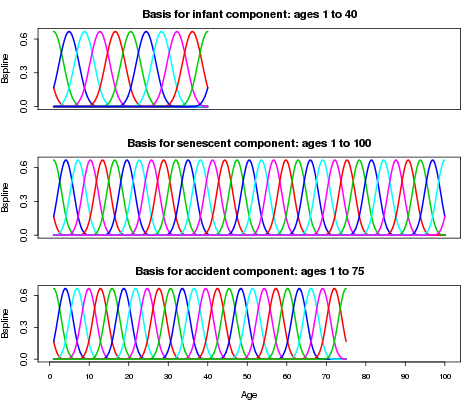
We call these additional penalties shape penalties to distinguish them from the usual smoothness penalties. The specific functional forms of Heligman and Pollard have been replaced with functions satisfying general smoothness and shape conditions. We illustrate the model with Swiss data for males aged 1 to 100 for 1980 taken from the Human Mortality Database. Figure 1 shows the bases of cubic \(B\)-splines for the three components. Notice that we make no attempt to impose any preconceptions on our bases. Thus, infant and child mortality can last to age 40, while the accident hump can extend from ages 1 to 75. The actual extent of both these components will be determined by our analysis, not by our assumptions.

This blog is not the place to describe the fitting process. We simply report the results. Figure 2 shows the observed and fitted mortality together with the three components, all plotted on the log scale. An important point is that the specific form of these components has emerged from the analysis, and not from the initial assumptions. In this sense, the CEG model can be seen as a generalization of the Heligman-Pollard model.

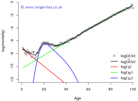
Figure 3 shows the observed, \(\boldsymbol{d}/\boldsymbol{e}\), and fitted, \(\boldsymbol{\hat d}/\boldsymbol{e}\), force of mortality on the original scale; the fit is evidently very good.

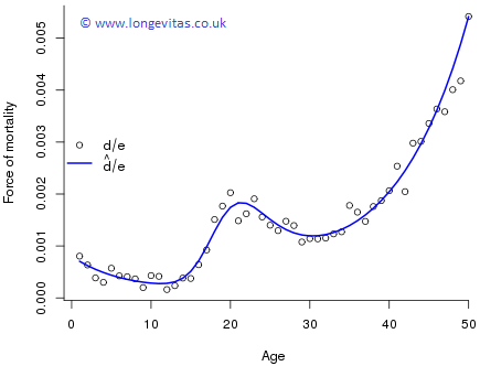
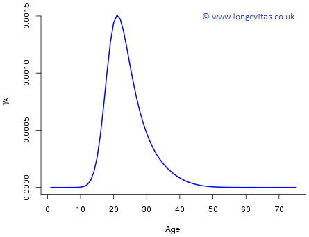
Figure 4 highlights the accident hump, \(\boldsymbol{\gamma_A}\), again on the original scale. The accident hump acts roughly from age 10 to age 50 with a sharp peak around age 20. The model enables the actuary to quantify in a precise way the additional risk over and above the underlying senescent mortality.

The search for the Holy Grail of a model for the mortality of the whole span of human life began with Gompertz (1825) and has had many significant contributions. One of the few to tackle the whole span was Heligman & Pollard's 1980 paper. Camarda, Eilers and Gampe, by generalizing the Heligman-Pollard model, is a further notable addition to this search.

Acknowledgement: I am extremely grateful to Giancarlo Camarda, Paul Eilers and Jutta Gampe for giving me access to their paper and for allowing me to bring this work to the attention of actuaries.

References:

Camarda, Eilers & Gampe (unpublished) Sums of smooth exponentials to model complex series of counts.
Eilers & Marx (1996). Flexible smoothing with B-splines and penalties, Statistical Science, 11, 89–121.
Gompertz, B. (1825). The nature of the function expressive of the law of human mortality, Philosophical Transactions of the Royal Society, 115, 513–585.
Heligman & Pollard (1980). The age pattern of mortality, Journal of the Institute of Actuaries, 107, 49–80.
Human Mortality Database. University of California, Berkeley, USA. Available at www.mortality.org (data downloaded January, 2016).
Jones (2005) web.stanford.edu/~jhj1/teachingdocs/Jones-mortmodel2005.pdf
R Core Team, (2015). R: A Language and Environment for Statistical Computing. Vienna: R Foundation for Statistical Computing.
Add new comment