A Model for Reporting Delays
In his recent blog Stephen described some empirical evidence in support of his practice of discarding the most recent six months' data, to reduce the effect of delays in reporting deaths. This blog demonstrates that the practice can also be justified theoretically in the survival modelling framework, although the choice of six months as the cut-off remains an empirical matter.
In our recent book, Modelling Mortality with Actuarial Applications, we introduce multiple-state models, and that is the framework we need here. Consider the model in Figure 1 for the death of a person observed from age \(x\), denoted by (\(x\)), with a delay in the death being reported.
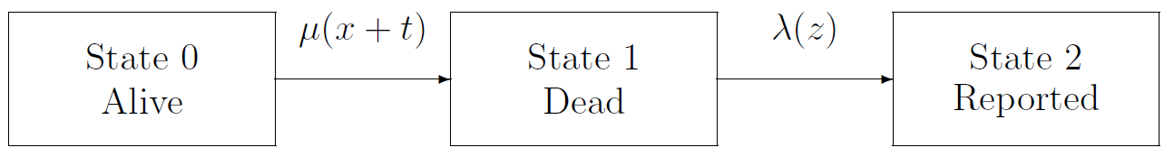
Define \(T_x\) to be the future lifetime of (\(x\)), and \(Z\) to be the time elapsed between death and the death being reported (conditional on death having occurred). We assume that the distribution of \(T_x\) is described by the hazard rate \(\mu(x+t)\), a function of age, and the distribution of \(Z\) (conditional on death having occurred) is described by the hazard rate \(\lambda(z)\), a function of the duration \(z\) since death occurred. We make two observations:
- The model is not Markov, because of the duration-dependence of the second transition.
- It is not difficult to assume that \(\lambda\) depends on age as well as duration, but we skip this for simplicity.
We define, as in Chapter 14 of our book, the occupancy probabilities \({}_tp_x^{00}\) and \({}_tp_x^{01}\), to be the probability that (\(x\)) is in state 0 (resp. 1) at age \(x+t\). Before death is reported, we know at time \(t>0\) that (\(x\)) is either in state 0 or in state 1, but which is unknown.
We define two counting processes, \(N^{01}(t)\) and \(N^{12}(t+z)\). (Recall that a counting process counts the number of the specified transitions that have occurred by the stated time, see Chapter 15 of our book. Here, since we are modelling an individual life, so these processes take values 0 or 1.) Death at age \(x+t\) is represented by \(dN^{01}(t)=1\), and the reporting of death at age \(x+t+z\) is represented by \(dN^{12}(t+z)=1\). Only the second of these is directly observable.
A marked point process (MPP) is a counting process where additional information, called a mark, is acquired when a specified transition takes place. We make our model a MPP by assuming that when a transition \(dN^{12}(t+z)=1\) occurs, we observe \(Z\) (which is equivalent to learning the value of \(T_x\)). Thus, \(Z\) is the mark.
The mark contributes an extra term to the likelihood. If \(dN^{12}(t+z)=1\), the contribution to the likelihood of the jump and the mark is:
\[\Pr[ \, dN^{12}(t+z)=1 \, ] \, \Pr[ \, Z=z \mid dN^{12}(t+z)=1\,] \qquad (1)\]
which is equal to the joint probability of the jump and the observed mark:
\[\Pr[ \, dN^{12}(t+z)=1 , Z=z \, ]. \qquad (2)\]
(Of course, this joint probability also admits the decomposition:
\[\Pr[ \, Z=z \, ] \, \Pr[ dN^{12}(t+z)=1 \mid Z=z \, ] \qquad (3)\]
but this has no useful interpretation in the survival models framework. Intuitively, we get to observe the mark because the jump has happened, not the other way round.)
Suppose \((x)\) is observed for time \(w\). In the case of a reported death, \(w=t+z\), otherwise \(w\) is some form of right-censoring time. We can now write down the likelihood in terms of the observed \(N^{12}(w)\). The likelihood, denoted by \(L\), is:
\[L = \left( {}_wp_x^{00} + {}_wp_x^{01} \right)^{(1 - N^{12}(w))} \, \left( \Pr[ \, dN^{12}(t+z)=1 , Z=z \, ] \right)^{N^{12}(w)}. \qquad (4)\]
The first term is the contribution of a censored observation (\(N^{12}(w)=0\)). The second term is the contribution of a reported death (\(N^{12}(w)=1\)).
The probability in equation (2) and the second term of equation (4) can be written as:
\begin{eqnarray*}\Pr[ \, dN^{12}(t+z)=1 , Z=z \, ] & = & \Pr[ \, T_x = t \, ] \, \Pr[ \, Z=z \mid T_x = t \, ] \\
&= &\exp \left( -\int_0^t \mu(x+s) \, ds \right) \, \mu(x+t) \, dt \\
& &\times \exp \left( -\int_0^z \lambda(s) \, ds \right) \, \lambda(z) \, dz\end{eqnarray*}
and the factors involving \(\lambda\) can be dropped from the likelihood for inference about \(\mu(x+t)\).
In conclusion:
- Contributions to the likelihood arising from reported deaths are the same as in the simple observable-death model, but with exponent \(N^{12}(w)\) (number of reported deaths) instead of \(N^{01}(w)\) (actual number of deaths).
- Contributions to the likelihood arising from censored observations include the occupancy probability \({}_wp_x^{01}\) in such a way that it cannot be factorized out, and the exponent involves \(N^{12}(w)\) instead of \(N^{01}(w)\).
Discarding the most recent data so that we may assume that \({}_wp_x^{01} \approx 0\) and \(N^{12}(w) = N^{01}(w)\) in most cases, in the retained data, is then a sensible approach. It yields approximately the correct likelihood:
\[L = \exp \left( - \int_0^w \mu(x+s) \, ds \right) \, \mu(x+w)^{N^{01}(w)}\]
since:
\[{}_wp_x^{00} = \exp \left( - \int_0^w \mu(x+s) \, ds \right)\]
(see equation (14.16) of our book, with appropriate changes to the notation).
This analysis does not, of course, tell us how much of the most recent data to discard, but Stephen's blog suggests that six months is an acceptable rule-of-thumb.
References:
Macdonald, A. S., Richards. S. J. and Currie, I. D. (2018). Modelling Mortality with Actuarial Applications, Cambridge University Press, Cambridge.

Add new comment