Forecasting with penalty functions - Part II
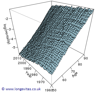
Our first blog in this series of three looked at forecasting log mortality with penalties in one dimension, i.e. forecasting with data for a single age. We now look at the same problem, but in two dimensions. Figure 1 shows our data. We see an irregular surface sitting on top of the age-year plane. Just as in the 1-d case, we see an underlying smooth surface, and it is this surface that we wish both to estimate and to forecast.
Figure 1: Crude log mortality rates for Australian males ages 50–90 over 1960–2010.
In the 1-d case we saw (a) how a basis of B-splines sat under the data, and (b) that each B-spline had a coefficient associated with the peak of its B-spline. The same idea applies in 2-d. Figure 2 shows (for a reduced data set) the grid of age-year locations for (a) data points, \(\circ\), and (b) coefficients, \({\color{blue}\bullet}\)
Figure 2: Age-year grid for (a) data \(\circ\) and (b) regression coefficients \({\color{blue}\bullet}\).
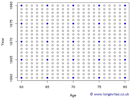
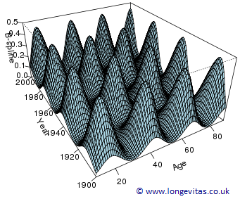
Figure 3 is a plot of a small basis of 2-d B-splines; the peak of each mountain sits directly above its location, \({\color{blue}\bullet}\), in Figure 2.
Figure 3: 2-d B-spline basis for ages 10–90 over years 1900–2000.
We note that this basis will tend to be quite large. In Figure 2 we have \(5 \times 4 = 20\) coefficients so the size of the basis is the product of the number of coefficients along the age and year axes. In our one-dimensional example we had 13 coefficients along the year axis so, in two dimensions, if we also had 11 coefficients along the age axis we would have a total of \(13\times11=143\) coefficients. In addition, we have 41 ages and 51 years so a total of 2091 observations. Evaluating each age-year grid point in turn at each 2-d B-spline we find our regression matrix, \(\boldsymbol{B}\), has size \(2091 \times 143\). Quite substantial!
I promised you some complications, so here is the first one. There is no natural order over a grid so we must impose one. When we form \(\boldsymbol{B}\) we assume that we vary age before year; i.e. the data are held in column order. With this convention in place we can fit a generalized linear model with log link, Poisson error and regression matrix \(\boldsymbol{B}\). Just as in the 1-d case, where an effective dimension of 13 resulted in over-fitting the data, we will also over-fit the data in 2-d with an effective dimension of 143. We will use penalized likelihood to bring about an appropriate level of smoothing.
The question is: how do we penalize in 2-d? Imagine the regression coefficients arranged in a grid, \(11 \times 13\), as in Figure 2. We penalize each row of the coefficient grid, i.e. the coefficients for each year for fixed age. We then repeat for a subset of ages what we did for single ages in 1-d. We use the same smoothing parameter in each row. This will bring about smoothness in time, but the surface may not be smooth across ages. We repeat the exercise by smoothing each column of coefficients. In other words, we smooth the surface by smoothing the coefficients in rows and columns. The penalized likelihood is $$\begin{equation} \label{eq:PL} \ell_p(\boldsymbol{\theta}) = \ell(\boldsymbol{\theta}) - \lambda_a \boldsymbol{\theta}^\prime \boldsymbol{P}_a \boldsymbol{\theta} - \lambda_y \boldsymbol{\theta}^\prime \boldsymbol{P}_y \boldsymbol{\theta} \qquad(1) \end{equation}$$ where \(\boldsymbol{P}_a\) and \(\boldsymbol{P}_y\) are penalty matrices in age and time respectively, and \(\lambda_a\) and \(\lambda_y\) are their corresponding smoothing parameters which jointly determine the amount of smoothing.
Figure 4: Observed and fitted profiles of log mortality for selected ages.
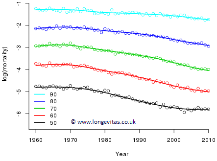
Figure 4 shows the result of maximizing \((1)\) for appropriate choices of \(\lambda_a\) and \(\lambda_y\). The effective dimension of the fitted model has been reduced from 143 (unsmoothed) to 55.2 (smoothed).
In contrast to the localised smoothing of this model, the likes of the Lee-Carter model is an example of a structural model, i.e. it imposes a structure on the mortality surface. One rather unsatisfactory feature of the Lee-Carter model is that the age profiles, i.e. those corresponding to Figure 4, all have precisely the same shape. By this we mean that the profile at age 60 in the Lee-Carter model can be transformed into the profile at age 70, say, by a simple change of location and scale! In contrast, the 2-d model presented here is a local model, by which we mean that the surface at a particular age and year is largely determined by the observations in its locality (the same remark applies to the 1-d P-spline model, of course, which was the basis of our free graduation tool).
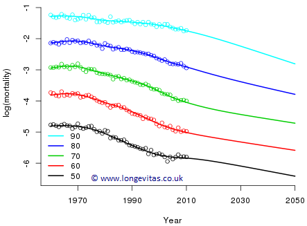
Finally, we turn to forecasting. One natural way of proceeding is to forecast the coefficients in each row of the estimated coefficient grid with the method we used so successfully in 1-d. This will result in linear forecasts at each age. However, I'm afraid this won't do; we can see from Figure 4 that the profiles are not parallel, so if we forecast linearly, the result will be crossover in mortality rates. In addition to the forecast in the year direction, we need something to keep the profiles apart, and to do so in a smooth fashion. This is exactly the function of the age penalty. So forecasting in 2-d is performed with precisely the same method as in 1-d: we define dummy deaths and exposures in the forecast region, and a weight vector with ones for observed values and zeros for missing values. As with the 1-d case, we fit and forecast all in one go (in contrast to the Lee-Carter model, where fitting and forecasting are two distinct stages). Figure 5 shows the result of this exercise. The forecasts look very reasonable, although special considerations apply when simulating sample paths from such penalty-projection models.
Figure 5: Observed, fitted and forecast profiles of log mortality for selected ages.
I promised you complications and we've only had one. In the next blog we'll look at some properties of 2-d forecasting. We've still plenty to discuss!
References:
Currie, Durban & Eilers (2004). Smoothing and forecasting mortality rates, Statistical Modelling, 4, 279–298.
Eilers & Marx (1996). Flexible smoothing with B-splines and penalties, Statistical Science, 11, 89–121.
Human Mortality Database. University of California, Berkeley, USA. Available at www.mortality.org (data downloaded 2015).
R Core Team, (2014). R: A Language and Environment for Statistical Computing, R Foundation for Statistical Computing, Vienna.
Add new comment