Forecasting with cohorts for a mature closed portfolio
At a previous seminar I discussed forecasting with the age-period-cohort (APC) model:
$$ \log \mu_{i,j} = \alpha_i + \kappa_j + \gamma_{j-i}$$
where \(\mu_{i,j}\) is the force of mortality at age \(i\) in year \(j\); the parameters \(\alpha_i\) , \(\kappa_j\) and \(\gamma_{j-i}\) are usually thought of as the age, period and cohort parameters respectively. These parameters are not identifiable from the formula above, so we need a set of constraints to fix unique estimates. Suppose we number the cohorts from 1 (oldest) to \(n_c\) (youngest). One set of constraints is as follows:
$$\sum \kappa_j = 0,\; \sum \gamma_c = 0,\; \sum c \gamma_c = 0.$$
Forecasting the mortality table now depends on forecasting the estimates of the period and cohort parameters. During the seminar I pointed out some difficulties with forecasting the cohort parameters, specifically the high correlation between parameters which are projected as though they are independent. This prompted the following question from the audience:
"Suppose we have a mature annuity portfolio closed to new entrants. Do we need to forecast the cohort parameters as we have all the years of birth we need?"
We can illustrate how this might work with Office for National Statistics (ONS) data on males for years 1961–2010. Assume that all the pensioners in our portfolio are 65 or older, so we use the age range 65–95 and we seek a mortality forecast to the year 2040, i.e. up to thirty years for the members of the portfolio. Notice that we forecast the full 30 years for the age 65 members but, for example, only 5 years for the age 90 members.
Figure 1. Data and forecast regions: ONS male data, ages 65–95, years 1961–2010, years of birth 1866–1945. Closed portfolio with youngest members age 65. Forecast thirty years to 2040. Figure 1 shows the data and forecast regions.
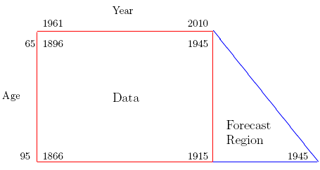
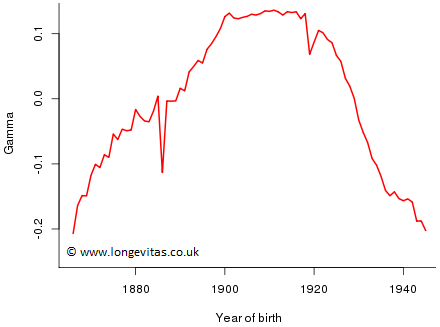
Figure 1 tells us that we have estimates of all the cohort parameters that we require, while Figure 2 tells us why we want to avoid forecasting the cohort parameters: continuing the clear trend in the estimates of the cohort parameters quickly leads to absurd estimates of mortality; alternatively, forecasting the estimates with a zero-drift time series also seems highly implausible.
Figure 2. Estimates of the cohort parameters for ONS male data with ages 65–95, years 1961–2010
Now the way forward is clear! Fix the age and cohort parameters at their estimated values and forecast the period parameters.
Is there a catch? Suppose the above solution is proposed by actuary A, while, independently, actuary B has the following thoughts:
- B is worried that the estimates of the younger cohort parameters are based on very little data, eg, the cohort parameter for an annuitant age 65 born in 1945 is based on a single data point (and so in this cell the observed and fitted deaths are exactly equal). Actuary B solves this problem by using ages 55–95.
- B also sees little point in going back to 1961 where the mortality pattern is rather different from more recent times. Actuary B solves this problem by using data from 1971–2010.
Figure 3: Estimates of \(\alpha\) by actuary A (red), by actuary B (blue)
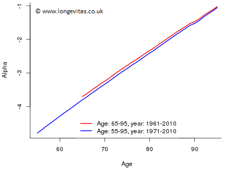
Figure 4: Estimates of \(\kappa\) by actuary A (red), by actuary B (blue)
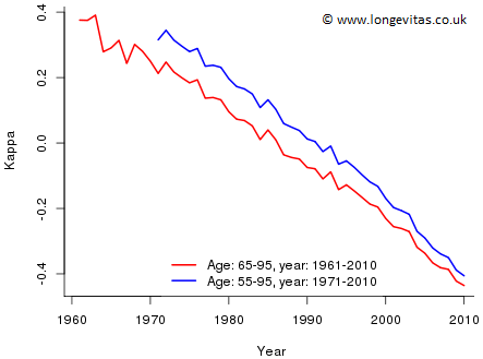
Figure 5: Estimates of \(\gamma\) by actuary A (red), by actuary B (blue)
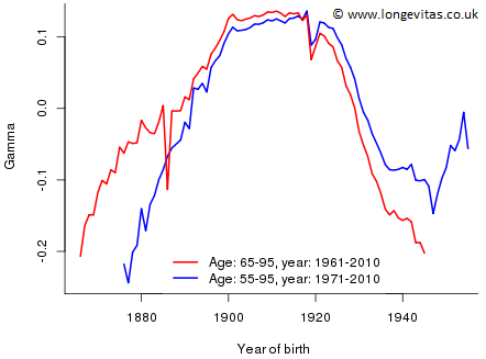
At first sight, Figures 3, 4 and 5 look a little disconcerting. The parameter estimates vary enormously depending on which data set is being used. However, we can reconcile the two approaches quite easily. The difference in the estimates of
- \(\alpha\) in Figure 3 is caused by actuary B excluding data with poorer mortality;
- \(\kappa\) in Figure 4 is caused by the constraint \(\sum \kappa_j = 0\) since actuary A centres around year 1985.5 while actuary B centres around year 1990.5;
- \(\gamma\) in Figure 5 is caused by the constraints \(\sum \gamma_c = \sum c \gamma_c = 0\) since actuary A centres around year of birth 1905.5 while actuary B centres around year of birth 1915.5
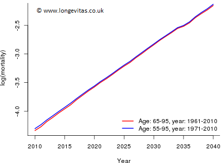
However, all is well since, for example, Actuary A estimates the log(mortality) of a male age 65 in 2010 as \(-4.34\) while Actuary~B estimates it as \(-4.30\). Indeed, the estimates of mortality made by A and B in 2010, the final year of observation, are very close for all ages. Thus both actuaries start their forecasts at the same values. From Fig 4 their forecasts of the period parameters are consistent and neither actuary needs to forecast age or cohort parameters. We conclude their forecasts of mortality will be consistent and the use of different data sets has not made a significant difference to the forecasts, as illustrated in Figure 6 (the plots for other ages show a similar consistency).
Figure 6: Forecast of log mortality by actuary A (red) and actuary B (blue) for the cohort aged 65 in 2010
Our conclusion is that forecasting with the age-period-cohort model in a closed portfolio does successfully avoid the need to forecast the cohort parameters. Forecasting the cohort parameters in Figure 5 is not something I would undertake with any degree of confidence!
Comments
Thank you for this helpful blog post Iain. I agree with the rationale here - I see no reason why concerns about correlated parameters need force an actuary to rule out models with both cohort and period terms in the situation described.
In fact I believe it is possible to extend the arguement and apply it to open annuity portfolios when we are calculating measures that do not depend on assumptions about new business.
We might extend our ONS data so that we're including lives age 50 in 2010 (for consistency with your diagram). This would allow us to project with some confidence as far as the 1960 cohort.
Live born after 1960 (early 50s and younger) would not currently comprise material percentage of annuity liabilities - maybe 5% at most. So, perhaps with a small adjustment to reflect the additional uncertainty for the very young lives, an actuary may feel perfectly happy to use such a model to forecast mortality for the existing annuitants in an open portfolio.
I always get very nervous when the subject of forecasting with a model with a cohort term is proposed so I welcome the idea that it is possible to forecast with such a model without the need to forecast future cohort parameters. Nevertheless, this approach requires the inclusion of younger ages and this of necessity alters the estimate of the period term; the forecast depends fundamentally on the estimated period term. In my blog, Actuary B extended the age range to a limited extent and we didn't seem to encounter a problem, in the sense that A and B obtained very similar forecasts. I don't think this is the same thing as saying one has carte blanche to extend the age range à volonté.
Thanks Iain. This doesn't sound insurmountable then - in such a situation I might check the estimate of the period term for the extended range against that calculated using the ages I'm most interested in. If they aren't materially different (keeping in mind that even a small difference might compound up to something material over the projection period) then I can weigh up the slight change in the period estimate against my extra confidence in the cohort estimates (especially those with only a few observations) and decide how to proceed.
Thanks Iain. If memory serves, I believe the quoted question was mine! The blog post (and subsequent one) is very clear and the conclusion is comforting despite the uncertainties and complications associated with projecting models including cohort effects.
My view would be that the advantages of working with models including cohort effects far outweigh the disadvantages associated with models that do not. This would be despite the additional complexity and care required with the former.
Add new comment