Over-dispersion

Actuaries need to project mortality rates into the far future for calculating present values of pension and annuity liabilities. In an earlier post Stephen wrote about the advantages of stochastic projection methods. One method we might try is the two-dimensional P-spline method with the simple assumption that the number of deaths at age i in year j follows a Poisson distribution (Brouhns, et al, 2002). Figure 1 shows observed and fitted log mortalities for the cross-section of the mortality surface for age 70 with this method.

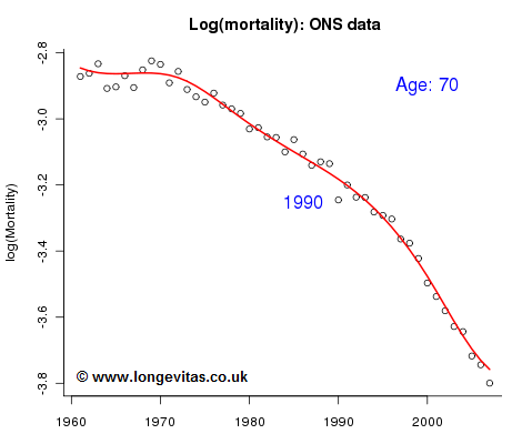
At first sight, all seems well - the fit seems perfectly reasonable and we could hope to forecast the fitted trend successfully. But there are two worrying features:

1. The smoothing parameters are 0 for age (yes, really) and 1 for year. This should set the alarm bells ringing since such low values of the smoothing parameters indicate a weak signal; volatile and unreliable forecasts are a likely consequence.
2. How plausible is our Poisson assumption? Does the fitted curve provide a satisfactory smoothing of the observed rates? The standardised residuals should have an approximate N(0, 1) distribution, but at age 70 eight of the forty-seven residuals have an absolute value in excess of 3; the year 1990 is the worst offender with a residual of −6. This won't do: the observed variation from the fitted line is way in excess of what is reasonable under the Poisson assumption. The observed deaths are more variable than our Poisson assumption allows; this is the phenomenon of over-dispersion.

These two features have a catastrophic impact on the projections, as Figure 2 shows:

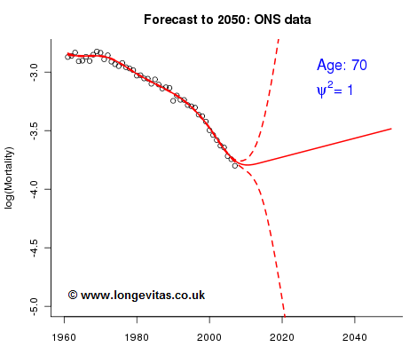
Figure 2 says it all - the forecast is hopeless. The alarm bells prepared us for things possibly going wrong but the scale of the disaster is still shocking.

The equality of the mean and variance of the Poisson distribution is the property that is letting us down. We need to relax this.  Can we fit a model which has the variance proportional to the mean?  To be precise, if D_i,j is the random variable representing the number of deaths at age i in year j we want:

Var(D_i,j) = Ψ²E(D_i,j)

where Ψ² is known as the over-dispersion parameter. The Poisson distribution fits neatly into this scheme with Ψ² = 1. We won't go into the technicalities of how such models are fitted here, but if you really want to see how it is done then have a look at Biatat & Currie (2009).

And what of the results of such a model? The estimate of Ψ² is 4.47, indicative of substantial over-dispersion and further confirmation that the Poisson assumption is well-wide of the mark here. Figure 3 shows the new cross-section for age 70, and this time everything is just as we would hope.

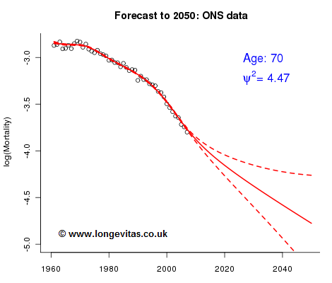
And what of our two alarm bells? The smoothing parameters, which were 0 and 1 when Ψ² = 1, are now 49 and 149 - a much stronger signal has been uncovered.  The residuals are also helped by the over-dispersion model.  At age 70, 1990 has once again the largest residual, but at -2.85 it is greatly reduced; only one other residual has an absolute value greater than 2. Over-dispersion has helped here too.

References:

Biatat, V. A. D. and Currie, I. D. (2009) On the problem of duplicates, Annals of Actuarial Science, Volume 5, Part 1, pages 33-52
Add new comment