Getting the rough with the smooth
There are two fundamentally different ways of thinking about how mortality evolves over time: (a) think of mortality as a time series (the approach of the Lee-Carter model and its generalizations in the Cairns-Blake-Dowd family); (b) think of mortality as a smooth surface (the approach of the 2D P-spline models of Currie, Durban and Eilers and the smooth versions of the Lee-Carter model).
In a time-series model the mortality rates of the population are presumed to follow an underlying process. But how do we simulate observed rates in a smoothed model which has no such process? In this post we describe how we can simulate future sample paths of mortality in this second family. An illustration from a smoothed model is shown in Figure 1.
Figure 1. Observed and fitted values for mortality at age 70 (left panel) and residuals (right panel). Source: Own calculations for 2D age-cohort P-spline model for the CMI assured-lives data with ages 40 to 89 and years 1950 to 2005.
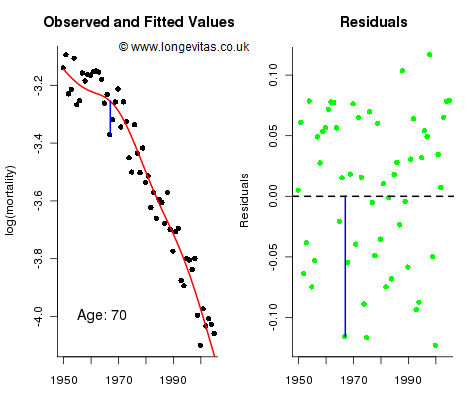
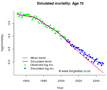
The left panel in Figure 1 shows the cross-section of observed and fitted mortality on the log scale for age 70; the right panel shows the unstandardised residuals which we collect in the matrix R = (r1, ... , rn ); here rj holds the residuals in the jth year. Figure 1 shows the residual at age 70 for 1967 in both panels. The fitted and forecast values of log mortality are described by the mean sheet, M, and its associated standard error sheet, S. Now let’s think about simulating future mortality. Let Z be an observation from the standard normal distribution N(0, 1). Then we account for parameter error with the forecast sheet M + Z × S. We can think of this forecast as the mean sheet lifted up (or down) by a random multiple of the standard error sheet; for example, if by chance Z=1.96, then the forecast sheet would be the upper 95% confidence sheet. Figure 2 shows the cross-section for age 70 for this process with Z=1.96; the mean forecast is in red and the upper 95% confidence forecast is in blue.
Figure 2. Observed and fitted mortality rates, together with best-estimate projection (red line) and simulated trend deviation (blue line). Source: Own calculations using model from Figure 1.
We have accounted for trend risk, so now we have to account for stochastic error. We use the matrix of unstandardised residuals, R. We assume that past residuals are representative of future residuals. For any future year we assume that the residuals are a random sample from the columns of R. This method of sampling has two important properties:
• It preserves ages, i.e. a future residual for age 70, say, will be a past residual for age 70. This is a desirable property since we expect the size of a residual to be age dependent — younger ages have fewer deaths and hence more variable residuals.
• It preserves years, i.e. the residuals of a future year are a random sample from the residuals of past years. This is another desirable property since it preserves such mortality shocks as may have occurred in the past. For example, 1963 was a very cold winter with consequent raised mortality; indeed, thirty-nine residuals out of fifty-six were positive. Our method of simulation allows these sort of shocks to occur again.
The results of adding stochastic error to the forecast are also shown in Figure 2. To sum up: simulating future sample paths in a smooth model of mortality is a two-stage procedure. First, simulate Z from N(0, 1), and second choose a random sample with replacement of size nF from the columns of R (where nF is the number of years to be forecast). The mean sheet, M, is then modified as described above for a trend error and an overlay of stochastic variation.
Add new comment