Back to the future with Whittaker smoothing

Many actuaries will be familiar with Whittaker smoothing (1923) but few will be aware of the close connection between this early method and the method of P-splines. The purpose of this blog is to explain this connection.

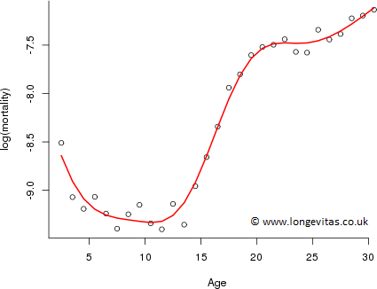
Figure 1 is a typical plot of log(mortality) of the kind of data we might want to smooth; here we use UK male data for 2011 for ages 2 to 30 taken from the Human Mortality Database.

Figure 1: Crude and Whittaker smoothed log mortality rates for UK males ages 2 to 30 in 2011.

Let \(y_i = \log(d_i/e_i), i = 1, \ldots, n\), be our data where the \(d_i\) are the observed deaths at age \(i\) and the \(e_i\) are the corresponding central exposures, and let \(\mu_i, i = 1, \ldots, n\), be the candidate smooth values of \(y_i\). Whittaker realizes that smoothing data is achieved by striking a balance between fidelity to the data and smoothness of the fitted curve. He defines fidelity and smoothness as follows: fidelity is measured by the sum of squares of deviations: $$\begin{equation} \label{eq:ssq} SS = \sum_1^n (y_i - \mu_i)^2 \end{equation}$$ and smoothness is measured "by the smallness of the sum of the squares of third differences" $$\begin{equation} \label{eq:smooth} \begin{split} M_3 = (\mu_4 - 3\mu_3 + 3\mu_2 - \mu_1)^2 + (\mu_5 - 3\mu_4 + 3\mu_3 - \mu_2)^2 \\ + \ldots + (\mu_n - 3\mu_{n-1} + 3\mu_{n-2} - \mu_{n-3})^2 \end{split} \end{equation}$$ Whittaker must now balance the relative sizes of \(SS\) and \(M_3\) which he achieves by considering $$\begin{equation} \label{eq:Balance} SS + \lambda M_3 \end{equation}$$ for some value of \(\lambda\). For a given value of \(\lambda\) our smooth curve is obtained by minimizing \((\ref{eq:Balance})\).

Back in 1923, the minimization of \((\ref{eq:Balance})\) for given \(\lambda\) required some pretty daunting arithmetic, certainly by today's standards. Nowadays we can easily write down an expression for an explicit solution and then use the power of a modern computer to evaluate it. We write \((\ref{eq:Balance})\) in matrix/vector form as $$\begin{equation} \label{eq:Matrix} ({\bf y} - {\bf \mu})^\prime ({\bf y} - {\bf \mu}) + \lambda {\bf \mu}^\prime {\bf D}^\prime {\bf D} {\bf \mu} \end{equation}$$ where \({\bf y} = (y_1,\ldots,y_n)^\prime\), \({\bf \mu} = (\mu_1,\ldots,\mu_n)^\prime\) and \({\bf D}\) is the third order difference matrix $$\begin{equation} \label{eq:D_3} {\bf D} = \left[\begin{array}{ccccccc} 1 & -3 & 3 & -1 & 0 & 0 &\cdots \\ 0 & 1 & -3 & 3 & -1 & 0 &\cdots \\ 0 & 0 & 1 & -3 & 3 & -1 & \cdots \\ \vdots & \vdots & \vdots & \vdots & \vdots & \vdots & \ddots \end{array} \right]. \end{equation}$$ Differentiating \((\ref{eq:Matrix})\) wrt \({\bf \mu}\) and solving, we have the Whittaker smooth for given \(\lambda\) is $$\begin{equation} \label{eq:W_soln} \hat {\bf \mu} = ({\bf I} + \lambda {\bf D}^\prime {\bf D})^{-1} {\bf y} \end{equation}$$ where \({\bf I}\) is the identity matrix of size \(n\). We would normally choose \(\lambda\) by minimizing AIC or BIC; Whittaker suggests that "we try two or three different values and see which gives the most satisfactory result". With 29 ages, equation \((\ref{eq:W_soln})\) requires the inversion of a \(29 \times 29\) matrix, far beyond what was possible in 1923. Whittaker found an explicit solution which was further simplified by Henderson (1924); the method is often referred to as Whittaker-Henderson smoothing, although the arithmetic remains challenging. We used trial and error directly with \((\ref{eq:W_soln})\); \(\lambda = 10\) gave a "satisfactory result" and the resulting smooth curve is shown in Figure 1.

So what is the connection between Whittaker smoothing and the method of P-splines (Eilers and Marx, 1996)? In a nutshell, Whittaker smoothing is a special case of the method of P-splines. In fact, the fundamental ideas in the Eilers and Marx paper are all in Whittaker's paper. In P-splines equation \((\ref{eq:W_soln})\) is replaced by $$\begin{equation} \label{eq:P_soln} \hat {\bf \mu} = ({\bf B}^\prime {\bf B} + \lambda {\bf D}^\prime {\bf D})^{-1} {\bf B}^\prime {\bf y} \end{equation}$$ where \({\bf B}\) is a regression matrix of B-splines of degree \(d\) (Eilers and Marx, 1996 equation (13)). If we use B-splines of degree zero with knot spacing of one year then \({\bf B} = {\bf I}\) and \((\ref{eq:P_soln})\) reduces to \((\ref{eq:W_soln})\)!

We mention four advantages of the P-spline method over Whittaker's method.

• We have additional flexibility with B-splines.
• We can use the P-spline method in a generalized linear model framework, which allows Poisson distributed deaths.
• Whittaker smoothing requires knot spacing of one year. With two dimensional data, this leads to challenging numerical difficulties. For example, if we have ages 50 to 90 and years 1950 to 2010 then equation \((\ref{eq:W_soln})\) requires the storage and inversion of a \(2501 \times 2501\) matrix. In contrast, with B-spline bases of degree \(3\) for age and year each with knot spacing of 5 years, then equation \((\ref{eq:P_soln})\) requires only the storage and inversion of a \(165 \times 165\) matrix.
• The efficient GLAM algorithms (Currie, Durban and Eilers, 2006) which may be used for P-spline smoothing are not available for 2-dimensional Whittaker smoothing.

So next time you smooth mortality data with P-splines just remember that you are essentially using the ideas that Sir Edmund Whittaker dreamed up nearly a century ago.

Footnote: If you want to try Whittaker smoothing for yourself you can find an R function and data as a downloadable zip file here ; the illustrative data will enable you to reproduce Figure 1. You can find further example smoothing code at our discussion of graduation. Note that R can be downloaded free of charge from the R website. If you need assistance in installing or running R, please see the list of frequently asked questions (FAQs). Neither Longevitas Ltd nor Iain Currie can supply support in installing or running R.

References:

Currie, Durban & Eilers (2006). Generalized linear array models with applications to multidimensional smoothing, Journal of the Royal Statistical Society, Series B, 6, 259–280.
Eilers & Marx (1996). Flexible smoothing with B-splines and penalties, Statistical Science, 11, 89-121.
Henderson (1924) A new method of graduation. Transactions of the Actuarial Society of America, 25, 29-53.
Human Mortality Database. University of California, Berkeley, USA. Available at www.mortality.org (data downloaded 2015).
R Core Team, (2015). R: A Language and Environment for Statistical Computing. Vienna: R Foundation for Statistical Computing.
Whittaker (1923). On a new method of graduation. Proceedings of the Edinburgh Mathematical Society, 41, 63-73.
Comments
Thanks for writing this. I'll be applying some version of this to baseline detection in signals.
Add new comment