Everything counts in large amounts

Models for projecting mortality are typically built using information on lives with deaths by age and gender. However, this ignores an important risk factor for longevity, namely socio-economic group. For annuity and pension reserving, therefore, it would be helpful to use such information when building stochastic projection models. Actuaries have two routes whereby they can get proxy information for socio-economic group: pension size and geodemographics.

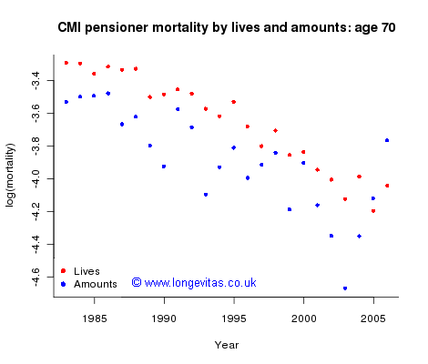
Typically such data is not available at the population level, but the CMI Pensioner dataset is one of the few with mortality data on both lives and amounts; we use these data for ages 60 to 90 and for years 1983 to 2006. Figure 1 shows observed log(mortality) for age 70. We make two remarks: (i) mortality by amounts is lighter than that by lives, and (ii) mortality by amounts is more volatile than that by lives. Neither of these points comes as a surprise to the actuary: the first is a truth universally acknowledged (by actuaries at least) and the second is easily explained: a single death generates multiple claims on a grand scale, namely the amount at risk for the life that died.

Figure 1. log(mortality) by lives and amounts at age 70. Source: CMI Pensioner data.

Suppose we have a model with a forecast for the data by lives. It is the purpose of this post to describe a simple method of adjusting this forecast in the light of the data by amounts. I have written earlier on piggyback models, which are a way of dealing with basis risk where company data suggest that using mortality datasets by lives will result in biased forecasts. However, piggyback models can also be used for our present problem. But before we use the piggyback model we will need to do something about the extreme volatility of the amounts data. The following method is well-known to many actuaries and goes back at least as far as Forfar et al. (1988). Let D^L, D^A, E^L and E^A be the matrices of deaths and exposures by lives and amounts. Then:

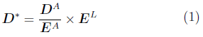
is an estimate of the number of deaths by lives if the underlying mortality is that by amounts. We can now write the piggyback model for amounts (with an obvious notation for elements of matrices) as:

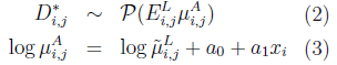
where x_i is the i^th age. Thus, on the log scale, the force of mortality by amounts μ^A is equal to the known force of mortality by lives μ^L adjusted by the term a₀ + a₁x_i. Note that this linear adjustment depends on age, but not on year; we’ll come back to this point in a moment. Figure 2 shows the result of fitting the model for age 70.

Figure 2. Piggyback model of log(mortality) by lives and amounts at age 70. Source: CMI Pensioner data.

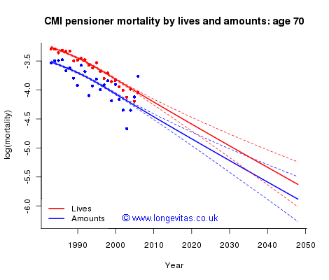
In our example, the model for mortality by lives was a 2d P-spline model with over-dispersion parameter, but any model which yields mean and standard-error sheets would do. The forecast by amounts for age 70 equals the forecast by lives lifted by a₀ + a₁x_i, where x_i = 70. We make two comments on Figure 2. First, the forecasts by lives and amounts are parallel; this means that the two forecasts are consistent in the sense that the forces of mortality by lives and amounts cannot cross over at some point in the future. Second, the forecast by amounts is essentially an adjustment for bias of the forecast by lives; the standard errors of the two forecasts are very close (although those for amounts are very slightly larger since the estimation of a₀ + a₁x contributes here).

Figure 3. Piggyback model of log(mortality) by lives and amounts at age 90. Source: CMI Pensioner data.

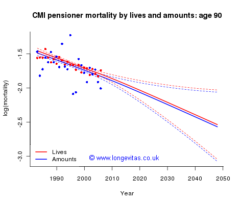
We make one final comment: the fitted linear adjustment in equation (3) was −1.030 + 0.0111 × age. At age 60 the adjustment is −0.365, a large adjustment which indicates a substantial difference between mortality by amounts and mortality by lives at this age (in Figure 2 the adjustment at age 70 is −0.254). However, at age 90 the adjustment has fallen to −0.032; there is little difference between mortality by amounts and mortality by lives at this age, as shown in Figure 3. This well-known phenomenon at older ages is sometimes called mortality convergence; see Gavrilov and Gavrilova (2001) and elsewhere.

Our example piggybacks the CMI amounts data on a fit to the CMI lives data. However, the piggyback model is a very general method of adjusting a given fit to data. For example, a company with just ten years of amounts data could use the above method to adjust any given fit to lives data; as usual, this could be split by rating factors if the company data allowed.

References:

Forfar, D.O., McCutcheon, J.J. and Wilkie, A.D. (1988). On graduation by mathematical formula. Journal of the Institute of Actuaries, 115, 1–149.
Gavrilov L.A., Gavrilova N.S. (2001) The reliability theory of aging and longevity. Journal of Theoretical Biology, 213, 527–545.
Add new comment