Another look at the Gompertz model

The year 1825 was a significant one not only for actuaries but for the wider scientific community: Benjamin Gompertz published his landmark paper on the graduation of human mortality (Gompertz, 1825). There were at least three completely new ideas in his paper. First, he gave his famous law of mortality. To quote Gompertz:

at the age \(x\) the intensity of man's mortality might be denoted by \(aq^x\)

or put another way, the logarithm of the force of mortality is linear in age. Second, the data he used was very limited and was available only at ten-year intervals; his law enabled him to interpolate between these given ages. Third, and this was significant for actuaries, he had a new way of valuing life contingencies.

Gompertz is something of a hero of mine. The originality of his mathematics is clearly compelling. He was largely self taught since, as a Jew, he was denied entry to university. There is a short biography available here that quotes Gompertz as seeing a mathematics book, while still a teenager, in the window of a bookseller. The bookseller was himself a mathematician and introduced him to the Spitalfields Mathematical Society which, as Gompertz later noted:

had many scholars then to teach, as one of the rules was, if a member asked for information, and applied to one who could give it, he was obliged to give it, or be fined one penny.

I thought it would interesting to see how the Gompertz law holds up nearly two hundred years since its publication. We will use UK male data for ages 50–90 and years 1970–2016 down-loaded from the Human Mortality Database. The data have the standard form: the number of deaths \(d_{x,y}\) at age \(x\) in year \(y\), and the central exposure or total time lived \(e_{x,y}\) at age \(x\) in year \(y\). Let \(\mu_{x, y}\) be the force of mortality at exact age \(x\) and exact year \(y\) but note that \(d_{x,y}/e_{x,y}\) is a point estimate of \(\mu_{x+1/2, y+1/2}\) since \(e_{x,y}\) is the central exposed to risk. Then for given year \(y\), the Gompertz law can be written

\[\log \mu_{x, y} = a + b x.\]

Figure 1. Observed and fitted log mortality with the Gompertz model for UK male data for ages 50–70 and years 1970, 1985, 2000 and 2016.

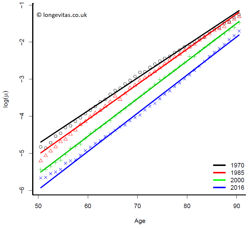
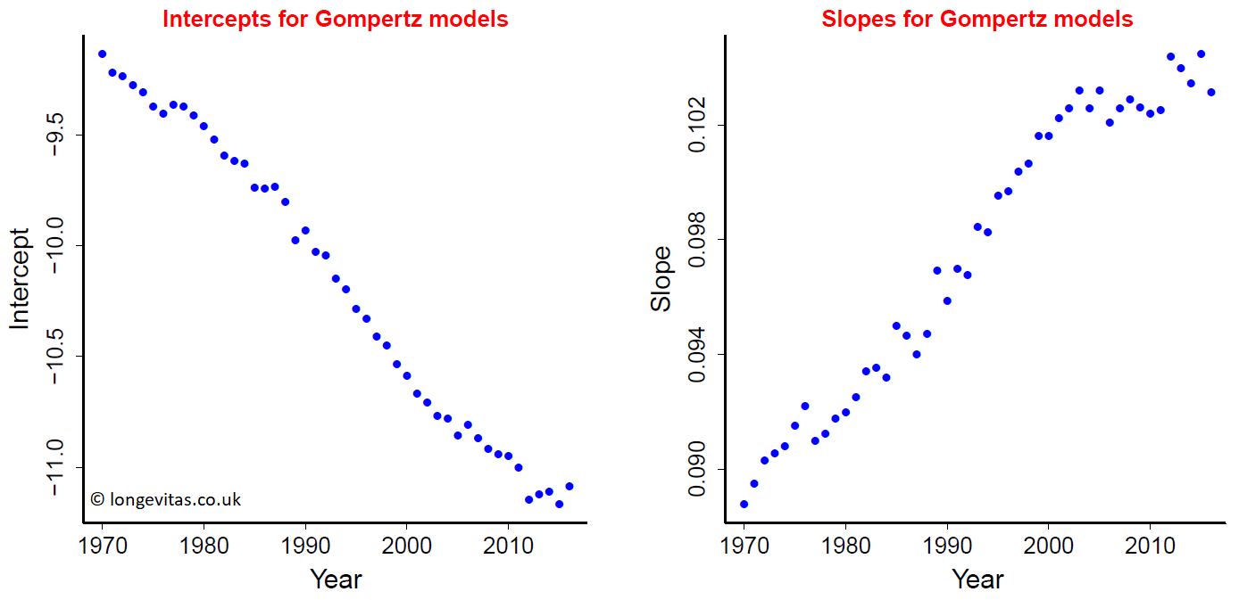
We assume that the number of deaths \(d_{x,y}\) follows the Poisson distribution and fit the Gompertz model for each year 1970–2016. We make some general comments. Figure 1 shows the results for 1970, 1985, 2000 and 2016. The improvement in mortality from 1970 to 2016 is very marked and well-known. Figure 2 plots the evolution of the parameters \(a\) and \(b\) over time.

• The plot of the intercepts, \(a\), in Figure 2 is nice and regular and suggests an improvement in mortality from year to year. This seems obvious but is perhaps falsely comforting since Figure 1 also shows the poor fit at the young ages at either end of the data period.

• The plot of slopes, \(b\), in Figure 2 is also nice and regular and suggests that the improvement just noted accelerates over time. Figure 1 reinforces this conclusion since the gap between the lines for 1970 and 1985 is smaller than the gaps between later lines.

• However, these two observations come with a caveat. The values of \(a\) and \(b\) in the later years in Figure 2 suggest that these improvements might have stalled over the last fifteen years.

Figure 2. Fitted values of intercepts \(a\) and slopes \(b\) from the Gompertz model fitted to UK male data for ages 50–70 and years 1970–2016.

We give a more detailed discussion of Figure 1. In 1970 the model over-estimates mortality at the younger and older ages and under-estimates it for the twenty years or so around age 70. A similar pattern is observed for year 1985 while the model fits rather well in 2000. In 2016 we see a reversal of the pattern in 1970 and 1985: the Gompertz model now under-estimates mortality at the younger and older ages while over-estimates mortality in the ages around 70. Of course, in itself this is not evidence of a systematic change in male mortality but it is suggestive.

Figure 3. Residuals \(\log \hat \mu_{x+1/2,y+1/2} - \log \dot \mu_{x+1/2,y+1/2}\) from the Gompertz model fitted to UK male data for ages 50–70 and years 1970–1990 (red) and years 2004–2016 (blue).

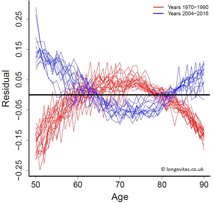
Figure 3 provides the evidence of this systematic change in the deviation from the Gompertz model over time. Let \(\dot d_{x,y}\) be the estimated number of deaths at age \(x\) in year \(y\) from the fits of the Gompertz models; let \(\hat \mu_{x+1/2,y+1/2} = d_{x,y}/e_{x,y}\) and \(\dot\mu_{x+1/2,y+1/2} = \dot d_{x,y}/e_{x,y}\) be the point estimates of mortality from the data and the Gompertz models respectively. The residuals of the observed and fitted log mortality are then \(\log \hat \mu_{x+1/2,y+1/2} - \log \dot \mu_{x+1/2,y+1/2}\). Figure 3 is a plot of these residuals. We see a clear pattern in the early years, 1970–1990 (coloured red), with the over-estimation of mortality at the younger and older ages and under-estimation for the central ages. The pattern is reversed for the later years, 2004–2016 (coloured blue).

I find this an intriguing finding. Inevitably this begs the question: what is the underlying change in male mortality that has brought about this change in the observed and fitted mortality? One partial answer may be the shifting distribution of exposure and deaths over the years. The Gompertz model has been fitted with the Poisson distribution for the number of deaths and a log link to ages. We have a generalized linear model or GLM. In such a GLM the weight given to individual data points equals the fitted number of deaths; Currie (2016, Table 10) gives a useful table of weights for various GLMs used in the modelling of mortality. In the present case, we find the mean of the fitted deaths over ages 50–52 and years 1970–1972 is 3,334 while over the same ages for the years 2014–2016 the mean is much lower at 1,340. In a similar way, the mean of the fitted deaths over ages 88–90 for years 1970–1972 is 3,325 while over the same ages for the years 2014–2016 the mean is much higher at 7,710. The model will follow the data more closely where the fitted deaths are higher, but will follow the data less closely where the fitted deaths are lower. This seems unlikely to be more than a very partial explanation. I suspect a full answer will not fit onto the proverbial postcard!

References:

Currie, I. D. (2016). On fitting generalized linear and non-linear models of mortality. Scandinavian Actuarial Journal, 2016, 356–383. doi: http://dx.doi.org/10.1080/03461238.2014.928230.
Gompertz, B. (1825). On the nature of the function expressive of the law of human mortality, and on a new mode of determining the value of life contingencies. Philosophical Transactions of the Royal Society of London, 115, 513–583.
R Core Team (2019). R: A Language and Environment for Statistical Computing. R Foundation for Statistical Computing, Vienna, Austria. URL https://www.R-project.org/.
Add new comment