Effective dimension

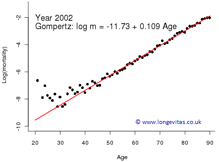
Actuaries often need to smooth mortality rates. Gompertz (1825) smoothed mortality rates by age and his famous law was a landmark in this area. Figure 1 shows the Gompertz model fitted to CMI assured lives data for ages 20–90 in the year 2002. The Gompertz Law usually breaks down below about age 40 and a more general smooth curve would be appropriate. However, a more general smooth curve would obviously require more parameters than the two for the simple Gompertz model.

Figure 1. Crude mortality rates (black dots) with fitted Gompertz line (solid red) on a logarithmic scale.

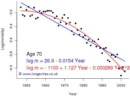
When we switch to a forecasting scenario, Figure 2 shows both a straight line and a parabola fitted to years 1947–2002 for age 70. Clearly, the quadratic curve gives a much improved fit, albeit at the (justifiable) expense of an extra parameter.

Figure 2. Crude mortality rates (black dots) with fitted straight line (solid blue) and alternative quadratic curve (solid red).

We use these two simple examples to introduce the idea of the dimension of a model. The Gompertz model in Figure 1 can be written as:

\[\log \mu_x = \alpha + \beta x\]

where x is age; this has two free parameters and we say the model has dimension 2. Similarly, the straight-line model in Figure 2 can be written as:

\[\log \mu_y = \alpha+\beta y\]

where y is year; as before, this has two free parameters and the model has dimension 2. The quadratic model in Figure 2 can be written as:

\[\log \mu_y = \alpha + \beta y + \gamma y^2\]

where y is year; this has three free parameters and the model has dimension 3.

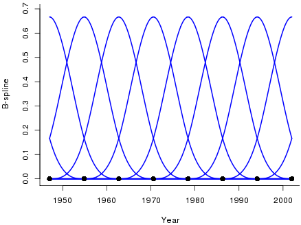
Many models for mortality use smoothing. The question then arises: can we attach a meaning to the dimension of a smooth model? Figure 3 shows a basis of ten cubic B-splines spanning the year range 1947 to 2002 (only part of the edge B-splines are shown).

Figure 3. A basis of ten overlapping cubic B-splines.

We can regress on this basis in exactly the same way as we regress on the bases in Figure 2: {1,y} in the straight-line model or {1,y,y²} in the quadratic model. The regression equation is:

\[ \log \mu_y = \sum_{j=1}^c B_j(y)\theta_j \]

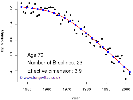
where c is the number of B-splines in the basis (c=10 in Figure 3). This model also has ten free parameters, one for each B-spline, so its dimension is ten. For our work we want a bit more flexibility than is given by ten splines, so Figure 4 shows the resulting fit with 23 B-splines in the basis. The model has dimension 23 which gives it great flexibility; however, a drawback of this flexibility is that the fitted curve is rather erratic. So how do we choose the number of B-splines in the basis to give the appropriate amount of smoothing? Too few B-splines will result in excessive smoothing and rigidity (as with the straight line in Figure 2), whereas too many B-splines cause under-smoothing (as in Figure 4).

Figure 4. Crude mortality rates (black dots) with fitted B-spline curve (red line) and B-spline coefficients (blue dots).

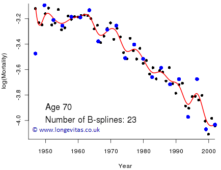
The fitted regression coefficients, θ_j, are plotted as a solid blue dot in Figure 4 with horizontal coordinate equal to the peak of its associated B-spline, B_j. The erratic nature of the fitted curve is a consequence of the erratic behaviour of the coefficients. The Eilers & Marx (1996) method of penalised splines (P-splines) will come to our rescue. This involves imposing a penalty function on the spline coefficients to make them behave more regularly. Figure 5 shows the result.

Figure 5. Crude mortality rates (black dots) with fitted penalised B-spline curve (red line) and B-spline coefficients (blue dots).

This looks very sensible but what is the dimension of this model? We still have 23 B-splines in the basis but the coefficients are no longer freely chosen; they are constrained to be smooth. If we apply very heavy smoothing then something very interesting happens: the fitted model tends to the straight-line of Figure 2! With no smoothing at all we have a model with dimension 23 and with very heavy smoothing we have a model with dimension 2. Our optimal model therefore has a dimension somewhere between 2 and 23; this dimension is called the effective dimension of the model. We do not discuss the detail here, but in Figure 5 our model has an effective dimension of 3.9; we can think of this model as being roughly equivalent to fitting a cubic (with exact dimension 4) but which makes better use of the available dimension.

Targetting a given level of smoothness reduces the effective dimension of the model. However, we can turn this whole process round, i.e. specify the effective dimension and work out the necessary level of smoothing. For example, we could use a basis of 23 B-splines and then specify a model with an effective dimension of 5, say. We talk about targetting the effective dimension. Why might you want to do this? The actuary is interested in forecasting mortality in 2-dimensions. The above argument extends to two dimensions where we might target an effective dimension in the range 15 to 30, say. The optimal fit would probably have a far greater dimension than this, and so have much greater flexibility. However, this flexibility might result in a very volatile forecast; one way of controlling the volatility of the forecast is to specify an effective dimension. However, this is no free lunch: the resulting confidence intervals may be optimistically narrow.

References:

Gompertz, B. (1825) The nature of the function expressive of the law of human mortality, Philosophical Transactions of the Royal Society, 115, 513–585.
Eilers, P. H. C. and Marx, B. D. (1996) Flexible smoothing with B-splines and penalties, Statistical Science, 11, 89–121.
Add new comment