Forecasting mortality at high ages
The forecasting of future mortality at high ages presents additional challenges to the actuary. As an illustration of the problem, let us consider the CMI assured-lives data set for years 1950–2005 and ages 40–100 (see Stephen's blog posts on selection and data volumes). The blue curve (partly hidden under the green curve) in Figure 1 shows observed log(mortality) averaged over time. A striking feature of this curve is the suggestion of data-quality issues above age 95:
Figure 1. log(mortality) by age for CMI assured-lives data, ages 40-100.
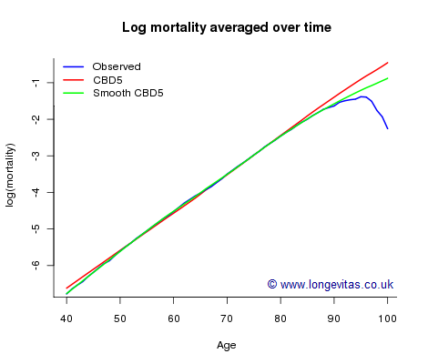
We don't believe mortality rates fall at high ages, so there must be a problem with the data. The obvious first solution is simply to model mortality up to an age where the data are credible. The drawback to this is that it leaves us without modelled mortality rates at the advanced ages. An alternative answer is to use a model with extrapolation for higher ages built into its structure. The following model for log mortality:
\[\log\mu_{i,j} = \kappa_{0,j}+\kappa_{1,j}(x_i-\bar x)\qquad(1)\]
is ideal for this purpose; here, \(\mu_{i,j}\) is the force of mortality at age \(x_i\) in year \(j\). This model is the fifth member of the extensive family of forecasting models described by Cairns et al. (2009); we will refer to it as CBD5. We can think of CBD5 as a collection of Gompertz models, one model for each year. The coefficients, the intercepts and slopes in the Gompertz models, with data restricted to ages 40–89 and years 1950–2005, are shown in Figure 2:
Figure 2. \(\kappa_0\) and \(\kappa_1\) parameters for CBD5 model fitted to CMI assured-lives data.

The left panel in Figure 2 shows how the general level of mortality has fallen over the last fifty years or so, while the right panel shows that the rate of change (slope) of mortality with respect to age has increased over time. Figure 2 suggests that it should be possible to forecast \(\kappa_0\) and \(\kappa_1\); Cairns et al. used a bivariate random walk with drift for the forecasting. With the forecast values of \(\kappa_0\) and \(\kappa_1\) in place, expression (1) yields a forecast for the whole mortality table. We can now see why CBD5 is so well suited to forecasting in the age direction. First, we fit CBD5 with data in which we have confidence, say ages 40–89; second we perform the forecast, say to 2050; third, we assume that the model holds for ages 90–100. Expression (1) provides the fitted and forecast mortalities for the suspect ages 90 to 100. The fitted log(mortality) averaged over 1950–2005 for ages 40–100 (in red) has been added to Figure 1. The average Gompertz line (red) follows the data (blue) quite well up to around age 85; the model assumption increasingly over-rides the data above age 85.
Figure 1 suggests a possible improvement to CBD5. There is a systematic difference between the data and the Gompertz line, so we replace the linear function in age in (1) with a smooth curve:
\[\log\mu_{i,j} = \kappa_{0,j}+\kappa_{1,j}S(x_i-\bar x)\]
Readers of my earlier posts will guess what's coming next! We model the smooth curve with B-splines and penalties, the P-spline system of Eilers & Marx (1996). With (1) the linear function is easily extrapolated above age 89; with (2) the penalty function also enables this extrapolation to take place. Figure 1 shows that this model gives an improved fit (in green) over the region of the data (ages 40–89); above age 89, the extrapolation extends the fitted curve in a natural way. An important point is that this extrapolation does not depend in any way on data above age 89; the extrapolation for high ages follows the curve established with the data up to age 89. One agreeable consequence of this is that the extrapolation with the smooth CBD5 model (green) gives a compromise between extrapolation with CBD5 (red) and the data (blue).
Finally, what do the forecasts at higher ages look like? Figure 3 shows the data and our two forecasts:
Figure 3. Forecasts at age 95 for CMI assured-lives data under CBD5 model.
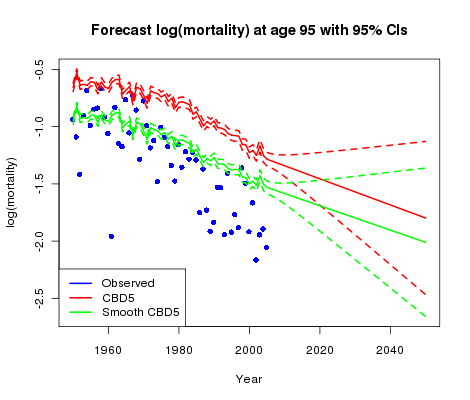
Both models show fitted log(mortality) higher than observed mortality at age 95; in line with Figure 1 the original CBD5 model gives larger differences from the data than the smooth version. The confidence intervals indicate a high level of uncertainly in the future direction of mortality — part of the price of forecasting without data!
There is a technical note (Currie, 2010) supporting this post.
References:
Cairns, Blake, Dowd, Coughlan, Epstein, Ong & Balevich (2009). A quantitative comparison of stochastic mortality models using data from England and Wales and the United States. North American Actuarial Journal, 13, 1–35.
Currie, I. D. (2010). A note on a model of Cairns, Blake and Dowd.
Eilers & Marx (1996). Flexible smoothing with B-splines and penalties. Statistical Science, 11, 89–121.
Add new comment