Fun and games with constraints

I'm a statistician so I worry about standard errors just as much as I worry about point estimates. My blog Up close and intimate with the APCI model looked at the effect of different constraints on parameter estimates in models of mortality. This blog looks at the effect of constraints on the standard errors of the parameter estimates. The results for standard errors are equally surprising as those for parameter estimates; we even have an example where a standard error is identically zero. Both sets of results serve to remind us exactly what is meant by not identifiable.

We will illustrate the ideas with the age-period-cohort or APC model fitted to male data from the Office for National Statistics (ONS). We have the number of deaths, \(d_{x,y}\), age \(x\) last birthday in year \(y\) and corresponding mid-year population estimates, the central exposures \(E^c_{x+1/2, y+1/2}\), for ages 50 to 104 and years 1971 to 2015. For convenience we use age indices \(1,\ldots,n_a\) and year indices \(1,\ldots,n_y\). We assume the oldest cohort in the first year is indexed 1 and so the cohort index at age \(x\) in year \(y\) is \(c(x,y) = n_a - x + y\). For our data we have \(n_a = 55\) ages, \(n_y = 45\) years and \(n_c = 99\) cohorts. We assume that the number of deaths follows a Poisson distribution with mean \(E^c_{x+1/2, y+1/2}\, \mu_{x+1/2, y+1/2}\) where \(\mu_{x+1/2,y+1/2}\) is the force of mortality at exact age \(x+1/2\) and exact year \(y+1/2\). The APC model is

\[\log \mu_{x+1/2,y+1/2} = \alpha_x + \kappa_y + \gamma_{c(x,y)},\,x = 1,\ldots,n_a,\,y = 1,\ldots,n_y.\qquad(1)\]

The APC model is not identifiable, by which we mean that we cannot find unique estimates of the parameter without further assumptions. These assumptions are usually in the form of constraints on the parameters; the following are often used (Cairns et al, 2009):

\[\sum_1^{n_y} \kappa_y = \sum_1^{n_c} \gamma_c = \sum_1^{n_c} c \gamma_c = 0. \qquad(2)\]

Now we do have unique estimates of the parameters. But what about their standard errors? The necessary formula is buried away in the Appendix to my 2013 paper in Statistical Modelling. The details can be found in the technical note supporting this blog.

Figure 1. Standard errors of \(\hat\gamma\) in APC model under constraints (2).

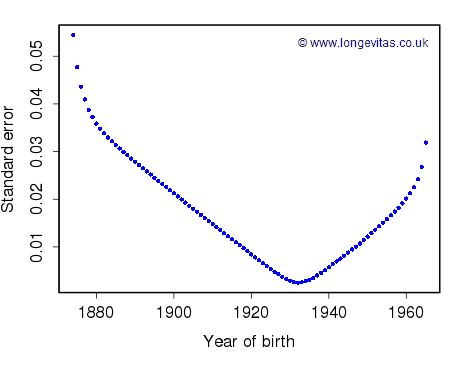
Figure 1 shows the standard errors of \(\hat\gamma\) under the constraints (2). There is nothing unexpected here. The general shape of the curve corresponds roughly to the number of cells in a particular cohort. In the corners for the young and old cohorts there are relatively few cells and we would expect high standard errors. Indeed, the standard errors for the very oldest cohorts are so large I have omitted them from the graph. These standard errors are the numerical evidence behind the practice of omitting corner cohorts in mortality models which include cohort terms.

Now things start to get interesting. What is the standard error of \(\sum_1^{n_c} \hat \gamma_c\)? We do the computation: answer 0. Of course it is. We have fitted the model subject to the constraint \(\sum_1^{n_c} \gamma_c = 0\) so the estimates satisfy the same condition identically and \(\sum_1^{n_c} \hat \gamma_c\) is estimated "without error".

Now let's make things really interesting. We know from our work on invariance that fitted and forecast values of mortality are invariant with respect to the choice of constraints; see Currie (to appear). This result holds provided we use an \({\rm ARIMA}(p, d, q)\) model, \(d = 1, 2\), with a fitted mean. Here is an equivalent set of constraints:

\[\sum_1^{n_y} \kappa_y = \gamma_1 = \gamma_c = 0. \qquad(3)\]

Figure 2. Standard errors of \(\bf\hat\gamma\) in APC model under constraints (3).

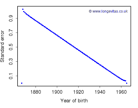
Figure 2 shows the resulting standard errors. They have a completely different shape from those in Figure 1. We note in particular that the standard errors of \(\hat \gamma_1\) and \(\hat \gamma_{n_c}\) are exactly zero. Should we worry? Of course not. When we come to forecasting mortality one set of constraints is as good as any other. The very different nature of the two sets of standard errors in Figures 1 and 2 shows that, just like the parameter estimates themselves, the standard errors are not identifiable. But there is more. The standard errors of the fitted values of mortality are identifiable, just like the fitted values themselves. Indeed, it would be very odd if two constraint systems which gave identical fitted values, gave different standard errors. There is a proof in the technical note.

What do we conclude from this exercise? There is a temptation to think of the constraints (2) (but not I think (3)) as a device to enable the estimation of the age, period and year of birth effects in order that they may be meaningfully forecast. This is simply not the case. The two sets of constraints are completely equivalent when it comes to the fitting and forecasting of mortality. If you insist on using (1) then you are making an assumption that the effects do indeed satisfy these conditions. This is a very strong assumption and one not easily checked.

I find this a very satisfying conclusion. Hunt and Blake (to appear) in a series of papers emphasize (a) the "arbitrary" nature of a particular set of constraints and (b) the importance of using a forecasting method which is invariant with respect to this arbitrary choice; they call such a method "well-identified". We completely agree with this position. It is said that "All roads lead to Rome"; in this blog "All roads lead to the unique fitted values of mortality, together with their unique standard errors".

References:

Cairns, A.J.G., Blake, D., Dowd, K., et al. (2009). A quantitative comparison of stochastic mortality models using data from England and Wales and the United States. North American Actuarial Journal, 13, 1-35.
Currie, I.D. (2013). Smoothing constrained generalized linear models with an application to the Lee-Carter model. Statistical Modelling, 13, 69-93.
Currie, I.D. (to appear). Constraints, the identifiability problem and the forecasting of mortality. Annals of Actuarial Science.
Hunt, A. and Blake, D. (to appear) Identifiability in age/period mortality models. Annals of Actuarial Science.
Hunt, A. and Blake, D. (to appear) Identifiability in age/period/cohort mortality models. Annals of Actuarial Science.
Hunt, A. and Blake, D. (to appear) A Bayesian approach to modelling and forecasting cohort effects. North American Actuarial Journal.
Add new comment