Model selection

When fitting a mortality model, analysts are faced with the decision of which risk factors to include or exclude.  One way of doing this is to look for the improvement in an information criterion that balances the fit against the number of parameters.  The bigger the improvement in the information criterion, the more strongly the model with the smaller value is preferred.

One natural question is "how big an improvement is significant?". In mortality models using individual lives we often use Akaike's Information Criterion (AIC), and in Macdonald et al (2018, page 98) we wrote that a difference of 4 AIC units could be regarded as a threshold. But where did the number 4 come from?

The answer comes from the concept of relative likelihood. If we regard the model with the smaller AIC (\(AIC_{min}\)) as having a likelihood of 1, the likelihood that a model with a larger AIC (\(AIC_{alt}\)) is actually correct is as follows:

\[{\rm Relative\ likelihood}=e^{(AIC_{min} - AIC_{alt})/2}\qquad(1)\]

Equation (1) is just an exponentially decreasing curve, as shown in Figure 1 below:

Figure 1. Relative likelihood by difference in AIC. Source: own calculations.

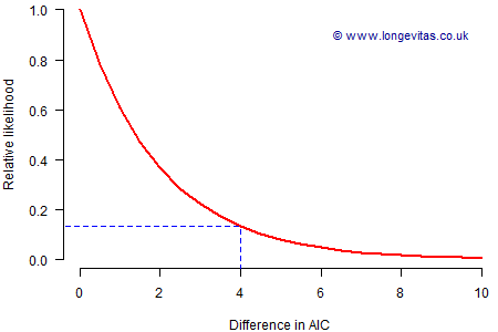
Figure 1 shows that the likelihood of the model with the larger AIC being the correct one tails off rapidly. Once the difference reaches 4 AIC units, the relative likelihood falls to 0.135 (\(=e^{-2}\)), which is a reasonable cut-off point (although different analysts may prefer other values).

The relative likelihood approach in Equation (1) and Figure 1 is very general and does not require the two models to be nested. An alternative approach is available if the two models are nested, i.e. one is a simplification of the other, and the parameters are not near boundary values. For such models one can use the Likelihood Ratio Test, which relies on Wilk's Theorem (Wilks, 1938). We assume that the model with the lowest AIC is the more complex model, and that the simpler model is a nested model with a higher AIC. With a little mathematics, we can write the difference in AICs as follows:

\[AIC_{simple}-AIC_{complex} = X-2n\qquad(2)\]

where \(X=-2\log\Lambda\). \(\Lambda\) is the ratio of the two likelihoods and \(n\) is the number of extra parameters in the alternative model. Under Wilk's Theorem, \(X\) has an approximately asymptotic \(\chi^2\) distribution with \(n\) degrees of freedom; the distribution functions for selected degrees of freedom are plotted in Figure 2, together with dashed blue lines showing the 95% quantiles.

Figure 2. Distribution functions of \(\chi^2\) distribution with varying degrees of freedom, and their 95% quantiles. Source: own calculations.

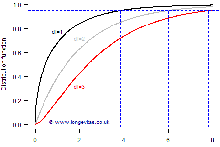
If we wanted to be at least 95% confident that the alternative model was truly better, then Figure 2 shows that the critical values for \(X\) are 4 for 1 degree of freedom, 6 for 2 degrees of freedom and 8 for 3 degrees of freedom. If we allow for the offset \(-2n\) in Equation (2), we get a common threshold value of 2 for the difference in AICs for one, two and three extra parameters. However, Wilk's Theorem relies on the likelihood having a quadratic shape around the MLE, and in certain cases the \(\chi^2\) distributional assumption might not hold true; to guard against this, one might use a higher threshold value than 2 to ensure that the true p-value wasn't lower than implied by the \(\chi^2\) assumption.

Of course, there are other considerations that drive model selection besides just fit. However, Figure 1 shows that a difference of 4 AIC units is a reasonable threshold.

References:

Macdonald, A. S., Richards. S. J. and Currie, I. D. (2018). Modelling Mortality with Actuarial Applications, Cambridge University Press.
Wilks, S. S. (1938) The large-sample distribution of the likelihood ratio for testing composite hypotheses, The Annals of Mathematical Statistics, Volume 9, No. 1, pages 60–62, doi 10.1214/aoms/1177732360.
Add new comment