Forecasting with limited portfolio data
In a recent post on basis risk in mortality projections, I floated the idea of forecasting with limited data and even suggested that it would be possible to use the method to produce a family of consistent forecasts for different classes of business. The present post describes an example of how this idea works in practice.
Forecasting with limited data depends on the simple idea of using actual portfolio data to adjust a separate forecast made with some very much larger reference data set. We use the following example:
- Reference data: CMI assured lives data between years 1950-2005, covering ages 40-89. We assume the data have been graduated and a forecast has been made to 2048, say. The output from this process consists of the graduated and forecast forces of mortality (on the log scale) together with their standard errors. We refer to these as the mean and standard error sheets. It doesn't matter how these sheets have been produced; our example uses the Lee-Carter method with smooth β and a time series forecast (this is the DDE method referred to in our earlier post on the Lee-Carter Family). Of course, you can use your own favourite method of forecasting.
- Portfolio data: we have pensioner data between years 2000-2007 at ages 60-95. Crucially, these data are classified by two factors: social class at two levels (high v. low social status, determined by geodemographic type) and pension size also at two levels (large v. small pensions).
Figure 1. CMI mortality rates at ages 75 and 76, together with rates observed in user portfolio at same ages.
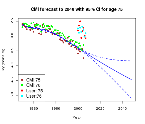
Figure 1 summarizes the situation. We see the CMI data for age 75 together with the graduation and forecast; the CMI data for age 76 are also shown. Everything is very tidy; the graduation and forecast are much as you would expect and the relation between the data at ages 75 and 76 is quite clear-cut. However, the portfolio data for ages 75 and 76 (averaged over the four sub-classes of business) carries no such clear message other than that the mortality of these pensioners is certainly heavier than that of the CMI assured lives.
Figure 2. log(mortality) by age for CMI reference data and four sub-classes of user portfolio data.
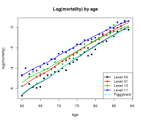
Something needs to be done. Figure 2 shows log(mortality) by age averaged over year for each of the four classes of business (blue, green, red and black dots); also shown is the corresponding log(mortality) for the CMI mean sheet (cyan line). Now we have something to get our teeth into! There is a pattern in Figure 2 which suggests that the gap between the portfolio data and the CMI sheet may be approximately linear in age.
Figure 3. log(mortality) by year for CMI reference data and four sub-classes of user portfolio data.
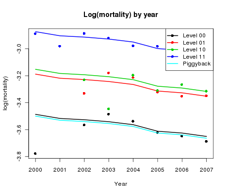
Figure 3 shows the corresponding plot by year averaged over age. How do the gaps behave this time? A reasonable and very simple assumption is that the gaps are constant in time. This is our key assumption since it allows us to adjust the CMI forecast by the simple expedient of estimating these gaps. The size of the gaps will depend linearly on age (according to our analysis of the previous paragraph).
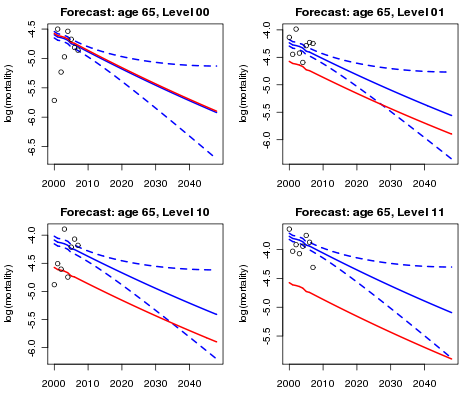
Now we are into the home straight! The assumption that the numbers of portfolio deaths have a Poisson distribution leads to a generalized linear model (GLM); forecasts for the mortality of our four classes of business together with their standard errors follow. The results of fitting the model have been added to Figures 2 and 3. Finally, Figure 4 shows the forecasts for age 65. The various adjustments made to the original forecasts based wholly on the CMI data are plain to see.
Figure 4. Reference forecast at age 65, together with piggy-back forecasts and 95% confidence intervals for each sub-class of the portfolio.
To sum up: we use the phrase piggyback model to describe the modelling and forecasting process since we "piggyback" our forecast on an existing graduation and forecast. Basis risk is an ever-present threat to the actuary; even when portfolio data does not support a stand-alone forecast, a piggyback model should remove some of this risk. And, as a bonus, any such adjustments can be fine-tuned to take account of the different risks associated with different classes of business.
Add new comment