The Lee-Carter Family
In a recent paper presented to the Faculty of Actuaries, Stephen Richards and I discussed model risk and showed how it can have a material impact on mortality forecasts. Different models have different features, some more desirable than others. This post illustrates a particular problem with the original Lee-Carter model, and shows how it can be combatted via smoothing. The choice of which parameters to smooth in the Lee-Carter model leads to a general family of models, which this note describes.
Let’s start by reminding ourselves of Lee and Carter’s original model (Lee & Carter, 1992), referred to here as LC. We’ll use the CMI data set with claims and central exposed-to-risk arranged in matrices D = (dij) and E = (eij) respectively; the rows are indexed by age of claim: 40, ... , 89, and the columns by year of claim: 1950, ... , 2005. LC assumed that:
log μij = αi + βiκj
where μij is the true, but unknown, force of mortality at age i in year j. The parameters in the equation above are not identifiable so we impose the constraints Σκj = 0 and Σκ2j = 1; these constraints have no effect on the estimated values of μij, nor on any subsequent forecast. LC’s idea is simple yet clever, since it reduces a 2-dimensional forecasting problem to the much simpler 1-dimensional problem of forecasting the time index, κ. Estimation is straightforward using maximum likelihood (Brouhns, Denuit & Vermunt, 2002) and Figure 1 shows the resulting parameter estimates, together with the observed and fitted log mortalities for age 70.
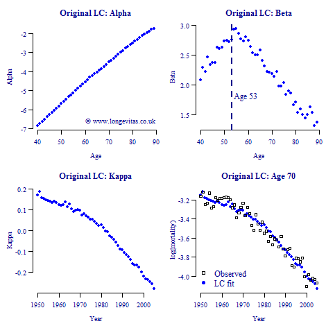
The idea behind our Lee-Carter family is to exploit the obvious regularities in the parameter estimates seen in Figure 1. This idea is not completely new: Delwarde, Denuit & Eilers (2007) (DDE) observed that irregularities in the estimates of the βi can have unfortunate consequences. The upper-right panel of Figure 1 shows a worrying jump between the estimate of βi at age 53 (low) and that at age 54 (high). This jump in the values of βi feeds through to the forecasts for ages 53 and 54 which crossover around year 2030, as the upper right panel of Figure 2 shows.
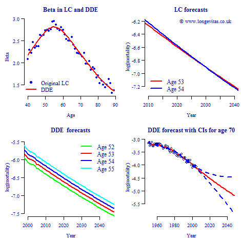
DDE dealt with this problem by smoothing the βi, and not surprisingly, they used the P-spline method of smoothing (Eilers & Marx, 1996); the upper left panel of Figure 2 shows the original LC β values and their smoothed values. The lower left panel in Figure 2 shows that not only has the crossover problem been solved but the mortality at successive ages progresses in a more regular fashion than in the original LC model. The lower right panel in Figure 2 shows the forecast at age 70 together with the 95% confidence interval.
But why stop at smoothing just β? The lower left panel in Figure 1 suggests that we could also smooth κ. We also use P-splines to smooth the κ, and as a bonus, the smoothing process itself also yields forecasts of the κ values; this has been widely described in the actuarial literature. We refer to this model as the Currie-Richards model (CR). The three models, LC, DDE and CR are the three models used in our paper on longevity risk referred to above.
Now that we have got a taste for parameter smoothing we can use a pick ’n’ mix approach. Models which don’t smooth κ forecast by time-series methods; on the other hand, models which do smooth κ use the smoothing process to forecast. Within these two sub-families we have various possibilities.
- Time-series sub-family. We already have two members: LC and DDE. If in addition to smoothing β, we smooth α, we have a third member, smooth Lee-Carter, and if we replace α by a linear function (the Gompertz law) we have what we call Gompertz-Lee-Carter.
- Smooth sub-family with forecasting via the smoothing process instead of a time series. To the existing CR model we can add the models with smooth or linear α.
If you’d like to see some of the theory behind these models and pictures of the output they give, then have a look at the slides from a talk I’ll give at the Actuarial Teachers’ and Researchers’ Conference at Queen’s University, Belfast next month.
Comments
am presently working on the model for my PhD THESIS in the university,i need to know more on the model
For more details on the model class, take a look at the links in the blog - there's a link to last year's paper at the start, and another link at the end to Iain's slides at a conference. Further conference presentations can be found at http://www.ma.hw.ac.uk/~iain/research/talks.html
Add new comment