Simulating the Future
This blog has two aims: first, to describe how we go about simulation in the Projections Toolkit; second, to emphasize the important role a model has in determining the width of the confidence interval of the forecast.
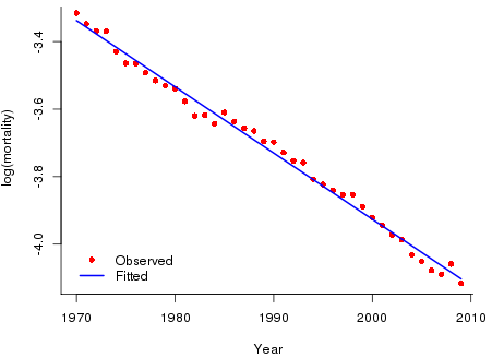
We use US male mortality data for years 1970 to 2009 downloaded from the Human Mortality Database. Figure 1 shows the observed log mortality. Unlike UK mortality (which shows accelerating improvements in log mortality over the same period) the US improvement is perfectly well described by a straight line. We fit the simplest of models: \(y_j = a + b x_j + \epsilon_j\), where \(x_j\) is year \(j\), \(y_j = \log(d_j/e_j)\) with \(d_j\) the observed number of deaths in year \(j\) and \(e_j\) the corresponding central exposed to risk; the error terms are independent \({\cal N}(0,\,\sigma^2)\). This is the familiar linear regression model. (Of course, these data are better modelled by a Gompertz model with Poisson errors but our purpose here is to keep things as simple as possible so that our main points are made clearly.) The fitted regression is also shown in Figure 1.
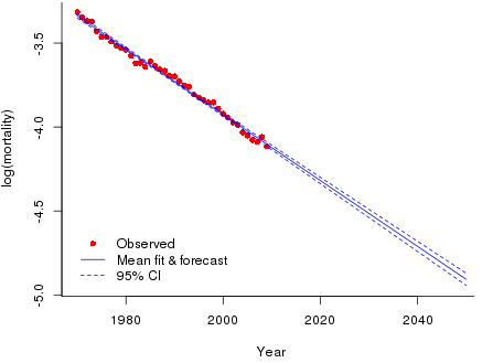
Suppose we wish to forecast log(mortality) to 2050. Forecasts in R are done with the \({\tt predict}\) function and importantly this function has the option of computing the standard error of both the fit and the forecast. Figure 2 show the fitted and forecast values with their standard errors. Readers may be surprised at the narrow confidence intervals. Intuitively, forecasts so far into the future should not be made with such apparent certainty. This is our second point. The width of the confidence interval is determined not only by the data but also by the model assumption. Here our data varies tightly around the fitted mean line so the estimate of the residual variance is small \((\hat \sigma = 0.022)\). We have also made a very strong model assumption and the strength of this assumption also leads to tight confidence intervals. Thus model risk affects not only the central forecast but also the confidence of that forecast.
We turn now to simulation. There are two ways of proceeding. The more obvious way is to simulate from the distribution of the estimates of the coefficients. If \(\boldsymbol{\theta} = (a,\,b)'\) then we have the well known result from linear regression that \(\hat {\boldsymbol{\theta}} \sim {\cal N}(\boldsymbol{\theta_0}, \sigma^2(\boldsymbol{X'} \boldsymbol{X})^{-1})\) where \(\boldsymbol{\theta_0}\) is the true but unknown value of \(\boldsymbol{\theta}\) and \(\boldsymbol{X}\) is the regression matrix. We can allow for the uncertainty in the estimation of \(\boldsymbol{\theta}\) by simulating values \(\boldsymbol{\tilde \theta}\) from \({\cal N}( \boldsymbol{\hat \theta}, \hat \sigma^2(\boldsymbol{X'} \boldsymbol{X})^{-1})\). Suppose \(\boldsymbol{\tilde \theta} = (\tilde a, \tilde b)'\) is a simulated value of \(\boldsymbol{\theta}\) then the simulated forecast at age \(x\) is \(\tilde a + \tilde b x\). The Toolkit uses a more direct method. We already know the fitted and forecast mean and its standard error, which we denote by the vectors \(\boldsymbol{m}\) and \(\boldsymbol {s}\) respectively; see Figure 2. The simulated value of the mean and the forecast is given by \(\boldsymbol{m} +\) \(z\boldsymbol{s}\) where \(z \sim {\cal N}(0,\,1)\). It is a simple matter to check that these two methods are precisely equivalent.
This is an important result as far as the Toolkit is concerned since it applies to time series models as well. With a time series model we obtain the mean forecast together with its standard error. Simulation can now proceed with the second method in the previous paragraph.
Of course, there are other things to worry about when simulating future mortality. The above method deals only with parameter risk. Both model risk and stochastic risk must also be accounted for. The Projections Toolkit has a selection of models to help with the former, and parameter risk and stochastic risk can be independently switched on and off as required within sample path generation. See my earlier blog for details.
References:
R Core Team, (2014). R: A Language and Environment for Statistical Computing. Vienna: R Foundation for Statistical Computing.
Human Mortality Database. University of California, Berkeley, USA. Available at www.mortality.org (data downloaded 2012).
Add new comment