Volatility v. Trend Risk

The year 1992 was important in the development of forecasting methods: Ronald Lee and Lawrence Carter published their highly influential paper on forecasting US mortality. The problem is difficult: given matrices of deaths and exposures (rows indexed by age and columns by year) can we forecast future death rates?  Lee and Carter designed a model specifically to solve this problem:

log μ_x,y = α_x + β_xκ_y        (1)

where α_x measures the average mortality at age x, κ_y measures the effect of year y; this year effect is modulated by an age dependent coefficient, β_x.  Lee and Carter used US data up to 1989 and here I’ve followed them by using data on US males aged 60–90 between 1933–1989, downloaded from the Human Mortality Database.

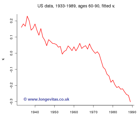
Now we see what they were up to.  If we assume that the α_x and β_x are stable in time then all we need to do is forecast the κ_y in Figure 1. The model has reduced forecasting a table to forecasting a one-dimensional time series.  Clever!

Now comes the tricky bit.  What time series do we choose?  Lee and Carter argued strongly from a plot similar to Figure 1 that the forecast should be based on a random walk with drift.  Thus:

κ_y = κ_y-1 + a + ε_y,   ε_y ˜ N(0, σ²),   y = 1934, ... , 1989          (2)

where the drift and volatility parameters a and σ are to be estimated from the values of κ_y in Figure 1.  We write this expression in terms of d_y = κ_y - κ_y-1:

d_y = a + ε_y,   ε_y ˜ N(0, σ²),   y = 1934, ... , 1989.

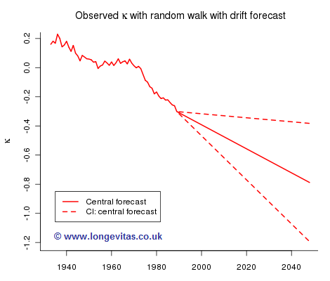
Our estimate of the drift parameter a is thus the mean of d_y, about −0.008 for these data; the estimate of σ² is the sample variance of d_y, which gives a standard error of about 0.003 for our drift parameter.  A very rough 95% confidence interval for a is (−0.014, −0.002) so a is not precisely determined.  This has alarming consequences for the accuracy of our forecast.  Figure 2 shows the best-estimate forecast for κ together with a 95% confidence interval:

Future sample paths generated by model (2) depend on both parameter risk and stochastic risk.  We can isolate stochastic risk and Figure 3 shows one hundred sample paths simulated under the assumption that the long term trend is fixed at the central forecast.  The dashed green line is the 95% envelope, i.e. the probability that the envelope contains a sample path is approximately 0.95.

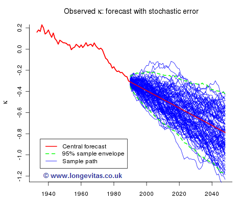
Figure 4 shows one hundred sample paths when only parameter uncertainty in the drift parameter is taken into account:

while Figure 5 shows one hundred sample paths when we allow for both  parameter and stochastic risk:

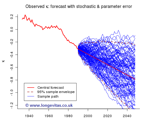
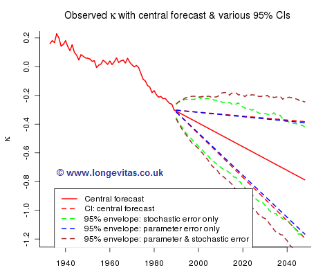
Figure 6 summarizes the relative contributions of parameter and stochastic risk:

Here are a few of the many comments that can be made on this exercise:

• Volatility is the dominant source of error in the short term.
• The importance of long term trend gradually increases over time until it eventually overtakes volatility as the “senior partner”.
• The mean-reversion property of the random walk with drift is obvious in Figure 3.  Are you comfortable that the course of future mortality behaves in this way?  I merely ask the question.

And a final question: is there an elephant in the room?  The above discussion assumes that the model is correct; there is no way we can be sure of this.  A cautious actuary will consider a range of models.  Only in this way can he or she come to an appreciation and understanding of longevity risk.

You can find some additional material in support of this blog in the technical note referenced below.