The cascade model of mortality
It is often instructive to look at mortality models where the parameters have an underlying meaning in a process. One interesting example of this is the cascade model of mortality, described by Izsak & Gavrilov (1995). Under the cascade model an individual in state \(n\) can do one of two things:
- Move to state \(n+1\) with intensity \(\lambda_0+n\lambda\), or
- Move to the dead state with intensity \(\mu_0+n\mu\).
where \(\lambda_0>0\) is the background rate of transition from one state to the next, \(\lambda>0\) is the additional rate of transition, \(\mu_0>0\) is the background rate of mortality and \(\mu>0\) is the additional rate of mortality. This is illustrated in Figure 1.
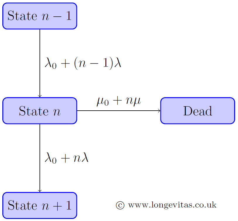
As is clear from the multiplier \(n\), the rate of transition from one state to the next becomes faster, and the rate of mortality increases as well. It is for this reason that the model is described as a cascade process. By letting \(n\to\infty\), Izsak & Gavrilov (1995) got the following expression for the force of mortality:
\[\mu(x) = \mu_0 + \frac{\mu\lambda_0\left(1-e^{-(\mu+\lambda)x}\right)}{\mu+\lambda e^{-(\mu+\lambda)x}}\qquad(1) \]
where \(\mu(x)\) is the force of mortality at age \(x\). As noted in Richards (2008, Appendix 3), if we assume \(\mu_0>\frac{\lambda_0\mu}{\lambda}\) we can make the following substitutions:
\[\eqalign{\epsilon &= \log\left(\mu_0-\frac{\mu\lambda_0}{\lambda}\right)\cr \beta &= \mu+\lambda \cr \rho &= -\log(\mu_0+\lambda_0) \cr \alpha &= \log \mu - \log \lambda + \log(\mu_0+\lambda_0)}\quad(2)\]
A spot of algebra then gives us this alternative expression for equation (1):
\[\mu(x)=\frac{e^\epsilon+e^{\alpha+\beta x}}{1+e^{\alpha+\rho+\beta x}}\qquad(3)\]
where \(\alpha, \beta, \rho\) and \(\epsilon\) are real-valued parameters to be estimated. The parameterisation in equation (3) is sometime called the Makeham-Beard model, and some estimated parameter values are given in Table 1.
Table 1. Estimated parameter values (MLEs) for 125,535 male pensioners in England & Wales (31,207 deaths).
| Parameter | Estimate |
|---|---|
| \(\hat\alpha\) | -13.2666 |
| \(\hat\beta\) | 0.131902 |
| \(\hat\epsilon\) | -5.07444 |
| \(\hat\rho\) | 0.0931642 |
In a survey of sixteen models in Richards (2012), I identified the Makeham-Beard model as the best-fitting for a set of annuitant-mortality data. Subsequent practical work has confirmed the usefulness of this model for general pensioner mortality. In other words, the simple four-parameter cascade process is equivalent to one of the best, all-round mortality models for annuitant and pensioner mortality.
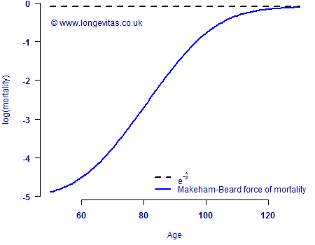
Izsak & Gavrilov (1995) observed that as \(x\to\infty\) in equation (1), the limiting force of mortality is \(\mu_0+\lambda_0\), i.e. that the limiting value for \(q_x\) is less than 1 under the cascade model. This is echoed in Greenwood (1926), who suggested that there is indeed a limiting value for \(q_x\), albeit one that is different for men and women. If we combine this insight with the substitutions in (2), we can see another interpretation of the so-called Beard parameter (after Robert Beard), \(\rho\), in equation (3): \(e^{-\rho}\) is the limiting force of mortality. This is illustrated in Figure 2.
References:
Greenwood, M. (1926) The natural duration of cancer, Reports on Public Health and Medical Subjects, Her Majesty's Stationery Office, 33, 1–26.
Izsak, J. and Gavrilov, L. A. (1995) A typical interdisciplinary topic: questions of the mortality dynamics, Archives of Gerontology and Geriatrics, 20, 283–293.
Richards, S. J. (2008) Applying survival models to pensioner mortality data, British Actuarial Journal, 14(II), 257–326 (with discussion)
Richards, S. J. (2012) A handbook of parametric survival models for actuarial use, Scandinavian Actuarial Journal, 2012 (4), 233–257.
Previous posts
Assumed or presumed?
Minding our P's, Q's and R's
I wrote earlier that deviance residuals were better than Pearson residuals when examining a model fit for Poisson counts. It is worth expanding on why this is, since it also neatly illustrates why there are limits to models based on grouped counts.
When fitting a model for Poisson counts, an important step is to check the goodness of fit using the following statistic:
\[\tilde{\chi}^2 = \sum_{i=1}^n r_i^2\]
Add new comment