Constraints: a lot of fuss about nothing?
Our paper, "A stochastic implementation of the APCI model for mortality projections", was presented at the Institute and Faculty of Actuaries in October 2017. There was quite a discussion of the role of constraints in the fitting and forecasting of models of mortality. This got me wondering if constraints weren't in fact a red herring. This blog is a short introduction to the results of my investigation into the role, or indeed the non-role, of constraints in modelling and forecasting mortality.
We illustrate our argument with data on UK males from ages 40–104 and for years 1961–2015 from the Office for National Statistics (ONS). We have the number of deaths, \(d_{x,y}\), age \(x\) last birthday in year \(y\) and mid-year population estimates, the central exposures \(E^c_{x+\frac{1}{2}, y+\frac{1}{2}}\); this gives a data matrix with \(n_x = 65\) rows and \(n_y = 55\) columns. We assume that \(D_{x,y}\), the random variable corresponding to the observed deaths \(d_{x,y}\), follows the Poisson distribution with mean \(E^c_{x+\frac{1}{2}, y+\frac{1}{2}}\, \mu_{x+\frac{1}{2}, y+\frac{1}{2}}\) where \(\mu_{x+\frac{1}{2}, y+\frac{1}{2}}\) is the force of mortality at exact age \(x+\frac{1}{2}\) and exact time \(y+\frac{1}{2}\).
The age-period model or AP-model is very simple, probably too simple to be useful, but it gives a clue as to why constraints might not matter. Under the AP-model we have:
\[ \log \mu_{x+\frac{1}{2}, y+\frac{1}{2}} = \alpha_x + \kappa_y,\; x = 1,\ldots, n_x,\; y = 1,\ldots, n_y.\qquad(1)\]
Notice that we are using the age and year index rather than the ages and years themselves; this will simplify the notation but makes no difference to the argument. This model is not identifiable, by which we mean that the parameters \(\boldsymbol{\alpha} = (\alpha_1, \ldots, \alpha_{n_x})^\prime\) and \(\boldsymbol{\kappa} = (\kappa_1, \ldots, \kappa_{n_y})^\prime\) are not uniquely estimable. The standard approach is to apply the constraint \(\sum \kappa_y = 0\) to the estimation in equation (1). Let us denote the maximum-likelihood estimates with this constraint by \(\boldsymbol{\hat\alpha}_s\) and \(\boldsymbol{\hat\kappa}_s\).
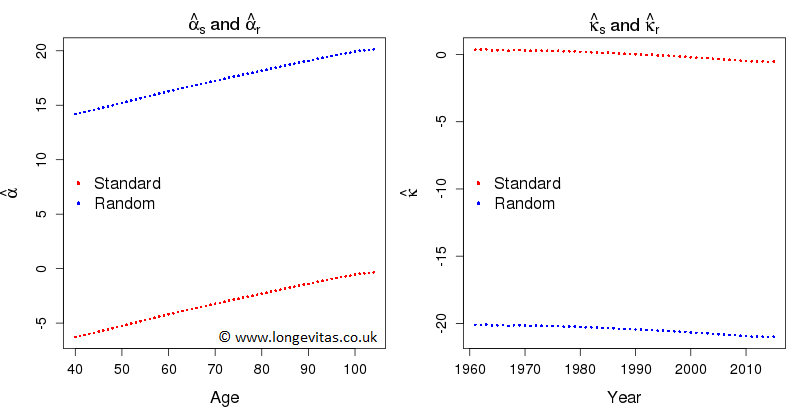
Now let's suppose that some perverse soul decides to apply a random constraint to \(\boldsymbol{\theta} = (\boldsymbol{\alpha}^\prime, \boldsymbol{\kappa}^\prime)^\prime\) by setting \(\sum u_i \theta_i = 0\) where \(u_i,\,i=1,\ldots,n_x+n_y\), are independent observations from the uniform distribution, \({\cal U}(0, 1)\). Let us denote the maximum likelihood estimates under this constraint by \(\boldsymbol{\hat\alpha}_r\) and \(\boldsymbol{\hat\kappa}_r\). Both sets of estimates are shown in Figure 1.
Figure 1. Estimates of \(\boldsymbol{\alpha}\) and \(\boldsymbol{\kappa}\) under the standard and random constraints.
1. The fitted forces of mortality under the two constraint systems are equal, i.e.
\begin{eqnarray} \log \hat \mu_{i,j} = \hat \alpha_{s,i} + \hat \kappa_{s,j} =\hat \alpha_{r,i} + \hat \kappa_{r,j},\;i = 1,\ldots, n_x,\, j = 1,\ldots, n_y.\end{eqnarray}
This is an example of a general property in a generalized linear model, namely, that the fitted values are invariant (unlike the regression coefficients, which are not).
2. The estimates \(\boldsymbol{\hat\alpha}_s\), \(\boldsymbol{\hat\kappa}_s\), \(\boldsymbol{\hat\alpha}_r\) and \(\boldsymbol{\hat\kappa}_r\) obey a very simple relation:
\[ \boldsymbol{\alpha}_r = \boldsymbol{\alpha}_s + k \boldsymbol{1}_x, \; \boldsymbol{\kappa}_r = \boldsymbol{\kappa}_s - k \boldsymbol{1}_y \]
for some real-valued \(k\), where \(\boldsymbol{1}_x\) and \(\boldsymbol{1}_y\) are vectors of 1s of appropriate lengths. In the diagram with the random constraints that I happened to use I found \(k = 20.47\). This should come as no surprise, since it corresponds to adding \(k\) to \(\alpha_x\) and subtracting \(k\) from \(\kappa_y\) in equation (1).
3. Forecasting in the AP-model is done by forecasting the \(\kappa\) values, keeping the \(\alpha\) values fixed at their estimated values and then using equation (1) to forecast the log mortality at each age. A moment's thought tells us that the forecast log mortalities under either constraint system will be equal since the change in the \(\kappa\) forecast is exactly compensated for by the change in the \(\alpha\) values.
Thus, the fitted and forecast values of log mortality are invariant under changes in the constraints used to make the parameter estimates identifiable. We are interested in the parameter estimates only insofar as they enable us to forecast the log mortalities. We conclude that we can use any constraints we like: we will always end up with the same forecasts.
You would be forgiven for thinking that this is a one-off example and arises out of the simple form of the AP-model. However, this is very far from the case and the same invariance result applies to, for example, the age-period-cohort model, the cohort extension to the Cairns-Blake-Dowd (CBD) model and even to the recent CMI APCI model. We illustrate with a look at a non-trivial example, the CBD model with added cohort effects; see model M6 in Cairns et al. (2009):
\[ \log \mu_{x+\frac{1}{2}, y+\frac{1}{2}} = \kappa^{(1)}_y + \kappa^{(2)}_y(x - \bar x) + \gamma_{n_x + y - x},\; x = 1,\ldots, n_x,\; y = 1,\ldots, n_y.\]
Here we have indexed the cohorts, with the oldest cohort being cohort 1. Let \(\boldsymbol{\kappa}^{(1)} = (\kappa^{(1)}_1, \ldots, \kappa^{(1)}_{n_y})^\prime\), \(\boldsymbol{\kappa}^{(2)} = (\kappa^{(2)}_1, \ldots, \kappa^{(2)}_{n_y})^\prime\) and \(\boldsymbol{\gamma} = (\gamma_1, \ldots, \gamma_{n_c})^\prime\), \(n_c = n_x + n_y - 1\).
We follow the recipe laid out for the AP-model. The model requires two constraints to make the parameters identifiable. We use the constraints in Cairns et al. (2009), namely, \(\sum \gamma_c = \sum c \gamma_c = 0\) where \(c\) is the cohort index, \(c = 1, \ldots, n_c\); we also use two sets of random constraints on the \(n_x+3n_y - 1\) parameters. We denote the two sets of estimates by the suffix \(s\) (standard) and \(r\) (random).
Figure 2. Differences in parameter estimates under standard and random constraints: \(\boldsymbol{\kappa}^{(1)}_r - \boldsymbol{\kappa}^{(1)}_s\), \(\boldsymbol{\kappa}^{(2)}_r - \boldsymbol{\kappa}^{(2)}_s\) and \(\boldsymbol{\gamma}_r -\boldsymbol{\gamma}_s\).
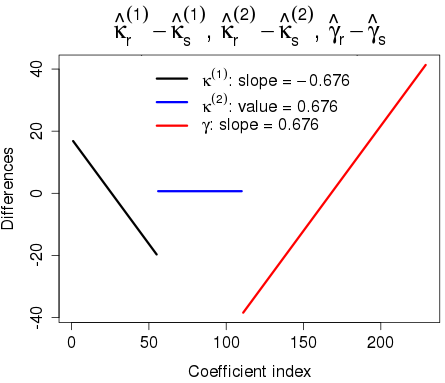
Figure 2 shows the relationship between the estimates under the two constraint systems. Just as in the case of the AP-model, this relationship has a very simple form. Indeed we can show that:
\begin{eqnarray} \boldsymbol{\kappa}^{(1)}_r &=& \boldsymbol{\kappa}^{(1)}_s + [A + (\bar x - n_x)B]\boldsymbol{1}_y - B\boldsymbol{y} \nonumber \\ \boldsymbol{\kappa}^{(2)}_r &=& \boldsymbol{\kappa}^{(2)}_s + B \boldsymbol{1}_y \\ \boldsymbol{\gamma}_r &=& \boldsymbol{\gamma}_s - A\boldsymbol{1}_c + B\boldsymbol{c} \nonumber \end{eqnarray}
where \(\boldsymbol{1}_y\) and \(\boldsymbol{1}_c\) are vectors of 1s of the appropriate length, \(\boldsymbol{y} = (1,\ldots,n_y)^\prime\), \(\boldsymbol{c} = (1,\ldots,n_c)^\prime\) and \(A\) and \(B\) are real-valued constants. For the random constraints used to obtain Figure 2 we found \(A = 39.1\) and \(B = 0.676\). The parameter estimates \(\boldsymbol{\hat\kappa}^{(1)}_s\) and \(\boldsymbol{\hat\kappa}^{(1)}_r\), and \(\boldsymbol{\hat\gamma}_s\) and \(\boldsymbol{\hat\gamma}_r\), are related by linear functions, while \(\boldsymbol{\hat\kappa}^{(2)}_s\) and \(\boldsymbol{\hat\kappa}^{(2)}_r\) differ by a constant: hence, the forecast with an ARIMA model with \(d > 0\), i.e. the order of difference greater than zero, will give the same forecast log mortalities. In particular a random walk with drift will be invariant to the choice of constraints.
When I set out to investigate the influence of constraint systems on forecasts, I had no idea that I would find myself back in the rarefied world of the linear algebra of my undergraduate days. But the fundamental results of matrix theory from that time were exactly what were needed to unlock the simple and, to my eyes at least, very beautiful results we have illustrated here. For those who would like to take a trip down memory lane and revisit their linear algebra course of yesteryear, you can find a general proof of the results used here in the technical note on the top right of this page; the two examples in this blog are used as illustrations of the general result.
These results on invariance also apply when some components of the model are smoothed (such as \(\boldsymbol{\alpha}\) in the AP-model). In this case some weak conditions must hold. You can get a flavour of these conditions from the slides of my talk on smoothing and invariance.
References:
Cairns, A. J. G., Blake, D., Dowd, K. et al. (2009). A quantitative comparison of stochastic mortality models using data from England and Wales and the United States, North American Actuarial Journal, 13, 1-35.
R Core Team (2017). R: A Language and Environment for Statistical Computing. R Foundation for Statistical Computing, Vienna, Austria. URL https://www.R-project.org/.
Richards, S. J., Currie, I. D., Kleinow, T. and Ritchie, G. P. (2017). A stochastic implementation of the APCI model for mortality projections, British Actuarial Journal (to appear).
Add new comment