A likely story

The foundation for most modern statistical inference is the log-likelihood function.  By maximising the value of this function, we find the maximum-likelihood estimate (MLE) for a given parameter, i.e. the most likely value given the model and data.  For models with more than one parameter, we find the set of values which jointly maximise the log-likelihood.

This much is basic statistics.  However, the log-likelihood function can give you more insight than just yielding MLEs.  In particular the shape and curvature of the log-likelihood tells you how much confidence you can have in a particular MLE.  By way of example, consider fitting a simple Makeham model for the force of mortality, μ_x:

μ_x = exp(ε) + exp(α + βx)

for which we can find the triplet of values for α, β and ε which jointly maximises the log-likelihood, and therefore provides the joint MLEs for the three parameters. We can also plot the log-likelihood for values around each parameter, which we do below for ε:

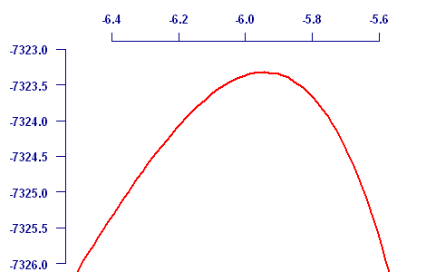
which shows that while the MLE for ε is -5.94, there is support for values in the interval (-6.40, -5.62) given the MLEs for α and β.  This suggests that the Makeham parameter for a constant background level of mortality is a valid model for this data set.  One of the handy things about support intervals is that they don't involve any further assumptions and don't have to be symmetric.  In the above example we can see that support on the right falls away faster than on the left.

The classical approach to statistical inference is to assume that the parameter estimate has a Normal distribution around the true value with a standard error of σ (say).  Thus, we would be 95% confident that the true value of ε in our example would lie within ±2σ of the estimated value.  The classical approach assumes a symmetric distribution around the true parameter value, and the usual means of doing this is to approximate the log-likelihood by a quadratic function.  We can see in the above graph that the log-likelihood is actually mildly skewed, but a quadratic approximation will be reasonable for the purpose of getting a rough standard error.

The problem with the classical approach is when the log-likelihood is neither symmetric nor approximately quadratic.  To illustrate this, consider the same profile log-likelihood for ε in the same Makeham model, but this time for a different data set where the Makeham parameter is not significant:

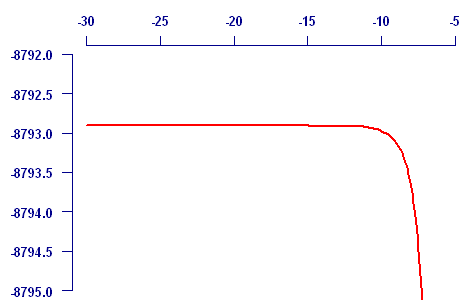
In this case the classical approach leads to a value for σ of 84,432, which is wildly larger than the likely values ε can take. This is caused by the log-likelihood being not remotely quadratic in shape, and certainly not symmetric.  The support-interval approach is more revealing, since the support interval for ε is actually (-infinity, -7.34).  This reflects the fact that the Makeham parameter is not significant, since exp(-infinity) is zero.