Mind the gap!
Recognising and quantifying mortality differentials is what experience analysis is all about. Whether you calculate traditional A/E ratios, graduate raw rates by formula (Forfar et al. 1988), or fit a statistical model (Richards 2012), the aim is always to find risk factors influencing the level of mortality.
Many such differentials are well-known and anticipated: females v. males, smokers v. non-smokers, healthy v. ill, rich v. poor. Each of these pairings has differentials large enough to merit their own mortality tables. And even where courts and politicians have regulated against straightforward pricing of observable differentials, such risk factors should still be acknowledged in reserving and risk management.
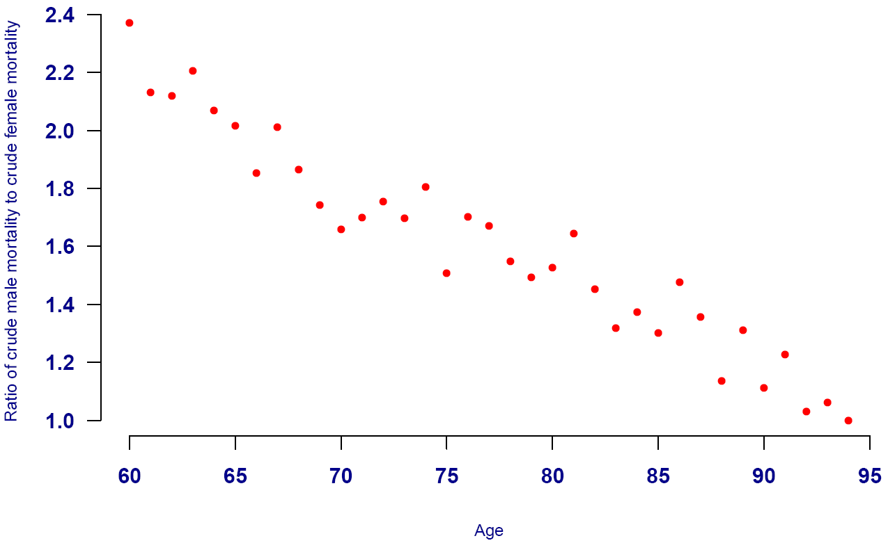
The reason why actuaries have developed separate mortality tables for the different risk classes is simple — you can't always use a single table shifted up or down by applying a single factor (qxnew = A * qxold). This does not allow for the fact that the difference in mortality between the two groups to be modelled is often age dependent. Take the example of males and females in Figure 1, which shows that the excess mortality for males decreases almost linearly with increasing age.
Figure 1. Ratio of crude male mortality hazard to crude female mortality hazard amongst UK annuitants. Source: Graph from Richards (2012).
The phenomenon of narrowing differentials with age is commonly referred to as mortality convergence, and is not confined to gender. In some instances the pattern is also more complex, as shown in Figure 2.
Figure 2. Crude mortality hazard for ill-health and normal retirements. Source: Data from Richards, Kaufhold and Rosenbusch (2013).
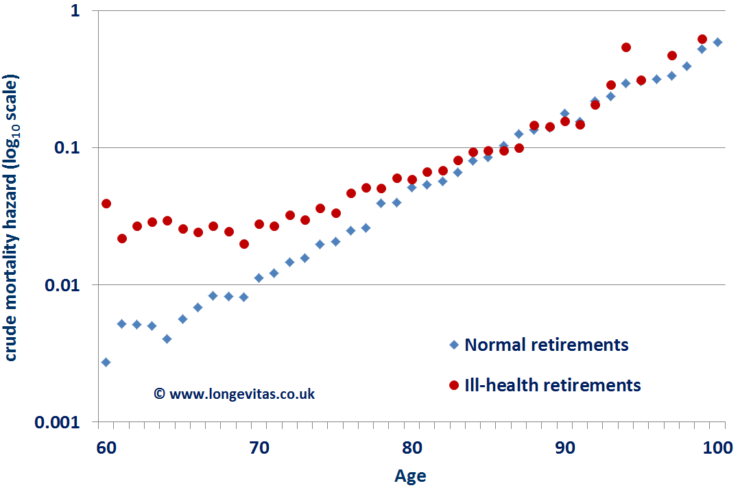
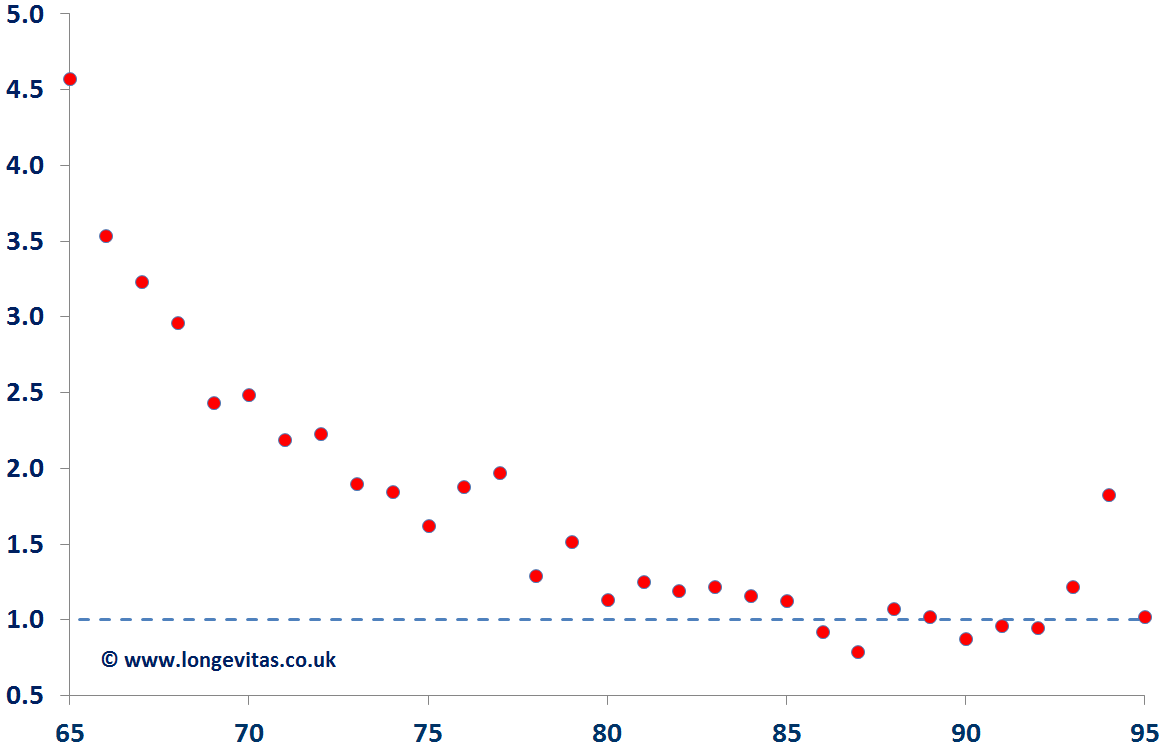
Figure 2 shows the crude mortality hazard rates for German pensioners. Excess ill-health mortality amounts to around 34 per mille for age 60, which then swiftly reduces to practically zero at age 85. Figure 3 shows the ratio of ill-health to normal pensioner mortality, which is suggestive of an exponential decay, rather than the linear run-off in Figure 1.
Figure 3. Ratio of crude ill-health mortality to crude normal-retirement mortality. Source: Data from Richards, Kaufhold and Rosenbusch (2013).
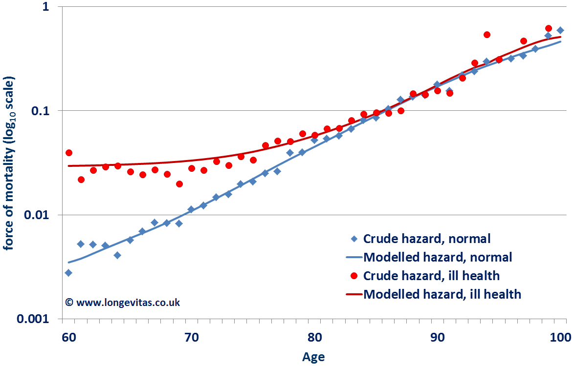
This age-dependent pattern of excess mortality is non-linear and explains why it is necessary to develop separate mortality assumptions for these two groups. However, often an actuary will be faced with the difficulty of not having enough data to develop a separate assumption for the smaller group on its own, and will therefore need to use the information contained in the rest of the dataset. In such circumstances, the actuary can use parametric models for the force of mortality, which allows both groups to be modelled and analysed simultaneously. In Figure 4 below, we see that the Makeham-Perks mortality law with different additive Makeham factors for ill-health and normal retirement has enough flexibility to match these two mortality patterns over a wide age range.
Figure 4. Crude hazard rates for normal and ill-health retirements, together with modelled rates. Source: Data from Richards, Kaufhold and Rosenbusch (2013).
Whether you are pricing life insurance or valuing pension liabilities, it is important to acknowledge that mortality differentials tend to narrow with increasing age. Of course, there will always be a need for actuarial judgement when there is little data available. However, using survival models can allow for several forms of age-dependent mortality differentials. And, as every Londoner knows, you have to be aware of gaps to avoid tripping over them!
References:
Forfar, D. O., McCutcheon, J. J. and Wilkie, A. D. (1988), On graduation by mathematical formula, Journal of the Institute of Actuaries, 115, 1–149.
Richards, S. J. (2012) A handbook of parametric survival models for actuarial use, Scandinavian Actuarial Journal, 2012 (4), 233–257.
Richards, S. J., Kaufhold, K. and Rosenbusch, S. (2013) Creating portfolio-specific mortality tables: a case study, European Actuarial Journal.

Add new comment