Minding our P's, Q's and R's

I wrote earlier that deviance residuals were better than Pearson residuals when examining a model fit for Poisson counts. It is worth expanding on why this is, since it also neatly illustrates why there are limits to models based on grouped counts.

When fitting a model for Poisson counts, an important step is to check the goodness of fit using the following statistic:

\[\tilde{\chi}^2 = \sum_{i=1}^n r_i^2\]

where \(r_i\) represents the residual for the \(i^{\rm th}\) Poisson count, usually a cell in a contingency table with \(n\) such cells. If the model is correct, the residuals \(\{r_i\}\) are usually assumed to be values drawn from the N(0,1) distribution. This in turn means that \(\{r_i^2\}\) are values drawn from the \(\chi_1^2\) distribution, and thus that \(\tilde{\chi}^2\) is a value drawn from the \(\chi_{n-k}^2\) distribution (\(k\) is the number of constraints or parameters estimated in the model). Comparing \(\tilde{\chi}^2\) against the appropriate percentage point of the \(\chi_{n-k}^2\) distribution then gives us our test of goodness of fit.

So, we have our testing edifice, but how sound is the foundation? In particular, how sound is the assumption that \(\{r_i\}\) are N(0,1)? We can test this via the simulation of Poisson variates using a known methodology, and then looking at the quantile-quantile plot of the two alternative definitions of residuals, i.e. Pearson and deviance. There is a function in R for this, \(\tt qqnorm()\), and if the residuals are normally distributed then the plotted points will form a straight line through the origin with slope 1.

We begin with the Pearson residual in Figure 1:

Figure 1. Normal quantile-quantile plots for Pearson residuals for 10,000 simulated Poisson counts with varying expected values (\(\lambda\in\{5,20,50,100\}\)).

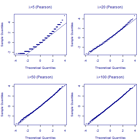
Figure 1 shows two features of Pearson residuals:

1. The quantile-quantile plots are only passably linear when \(\lambda\) gets to 100, i.e. the number of expected deaths in each cell of the contingency table needs to be over 50 (say).
2. The N(0,1) distribution is continuous, whereas the quantile-quantile plots show pronounced banding up to \(\lambda=20\).

The above observations are the reasoning behind the rule-of-thumb insistence that models for Poisson counts have at least 20 expected deaths on average. It is also clear that cells with 5 or fewer expected deaths are to be avoided wherever possible.

What about quantile-quantile plots for deviance residuals? These are shown in Figure 2 for the same simulated Poisson counts:

Figure 2. Normal quantile-quantile plots for deviance residuals for 10,000 simulated Poisson counts with varying parameter values (\(\lambda\in\{5,20,50,100\}\)).

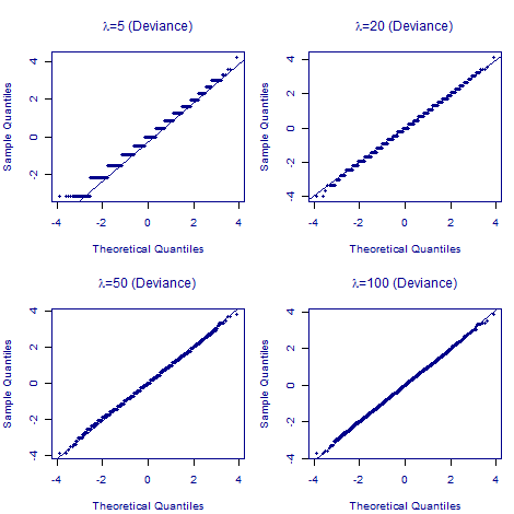
Figure 2 shows that the deviance residuals are better than Pearson residuals in all four cases; no matter the value of \(\lambda\), the quantile-quantile plot of deviance residuals is closer to a straight line of slope 1. We thus prefer the deviance residual in all cases, and certainly when the expected number of deaths is below 100.

However, Figure 2 also shows that deviance residuals are no panacea; if the number of expected deaths is below 20, the distribution is still not a continuous random variable, as shown by the step function in place of a straight line. While the deviance residual is a more reliable definition to use for the \(\tilde{\chi}^2\) test statistic, it is still important to avoid cells with fewer than five expected deaths. This needs to be borne in mind when fitting Poisson mortality models to grouped counts.