(Mis-)Estimation of mortality risk

One of the risks faced by annuity providers is mis-estimation, i.e. the risk that they have incorrectly assessed the current rates of mortality. This is often handled as a simple reduction factor applied to a published mortality table. There are two implicit assumptions behind this:

1. Mis-estimation risk is a constant proportion of mortality rates, and
2. Mis-estimation is a simple down-shift in rates without any offsetting aspects.

In fact the true situation is a lot more subtle than these two assumptions imply, as mortality risk can seldom be fully expressed with a single parameter. Richards et al (2013) demonstrated this with a multi-parameter model covering seven risk factors.

Multiple parameters in a model are almost inevitably correlated with each other. This can give rise to problems in parameter interpretation, or, in other cases, it can invalidate the assumptions of projection models. It is therefore important to analyse and understand parameter correlations when working with mortality models.

Parameter correlations can occur with even the simplest of models. For example, consider the two-parameter Gompertz (1825) survival model below:

\[\log \mu_{x_i} = \alpha_0+\beta_0 x_i \tag{1}\]

where \(x_i\) is the exact age of individual \(i\). The Gompertz model is a straight line on a logarithmic scale, where \(\alpha_0\) is the intercept of the line and \(\beta_0\) is the slope in age. Figure 1 shows the best-fit line in blue for a pension scheme in England & Wales:

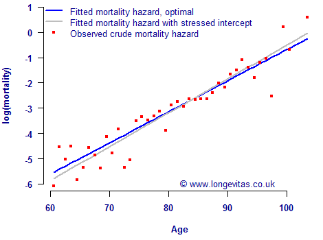
The best-estimate values of \(\hat\alpha_0=-12.972\) and \(\hat\beta_0=0.122872\) for the blue line in Figure 1 were determined by the method of maximum likelihood. As is standard for statistical estimation, this pair of estimates \((\hat\beta_0, \hat\alpha_0)'\) comes with a variance-covariance matrix:

\[\begin{pmatrix}3.18189\times 10^{-5} & -0.00261762\\-0.00261762 & 0.218081\end{pmatrix}\]

The leading diagonal of the variance-covariance matrix above tells the analyst about the error in estimation of the parameters. For example, \({\rm Var}(\hat\beta_0)=3.18\times 10^{-5}\), while \({\rm Var}(\hat\alpha_0)=0.218\). One of the handy things you can do with a variance-covariance matrix is to turn it into a matrix of percentage correlations between the parameters:

\[\begin{pmatrix}100 & -99.4\\-99.4 & 100\end{pmatrix}\]

The above matrix repays closer study. The leading diagonal is 100% because a parameter is obviously perfectly correlated with itself. The matrix is also symmetric about the leading diagonal because the correlation between \(\hat\alpha_0\) and \(\hat\beta_0\) must be the same as the correlation between \(\hat\beta_0\) and \(\hat\alpha_0\). What is interesting about the above matrix is the near-perfect negative correlation between \(\hat\alpha_0\) and \(\hat\beta_0\): -99.4%. This means that a change in the value of \(\alpha_0\) in the model would be accompanied by an offsetting change in the value of \(\beta_0\). This is shown by the grey line in Figure 1, where the value of \(\alpha_0\) has been stressed by deducting 1.96 standard errors and the value of \(\beta_0\) has been re-estimated. Figure 1 shows that a downward shift in the level of mortality, as represented by \(\alpha_0\), is accompanied by an offsetting change to the rate of increase with age, as represented by \(\beta_0\).

This situation has consequences for mis-estimation risk, i.e. the risk that an insurer has got its estimates of current (period) mortality rates incorrect. As Figure 1 shows, a simple downward shift in mortality level is too simple an approach. But is it possible to reduce these parameter correlations? To an extent it is — we first re-parameterise our Gompertz model as follows:

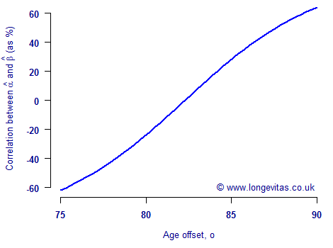
\[\log \mu_{x_i} = \alpha_0+\beta_0 (x_i-o)\tag{2}\]

where \(o\) is an offset age. Figure 2 shows the correlations between \(\hat\alpha_0\) and \(\hat\beta_0\) for varying values of \(o\). The correlation between the two parameters is reduced to -3% at age 82, and is zero just above this age. We say that we have orthogonalised the model by restructuring it so that parameter correlation is minimised.

So, does this mean that we can eliminate parameter correlations by restructuring our models? Unfortunately not — this orthogonalising trick only works for the very simplest of models. For example, consider what happens when we extend the model in (2) to include gender as a risk factor:

\[\log \mu_{x_i} = \alpha_0+\alpha_{male}I_{male,i}+\beta_0 (x_i-o)\tag{3}\]

where \(\alpha_{male}\) represents the additional risk of being male and \(I_{male,i}\) is an indicator variable which takes the value 1 for males and 0 for females. With \(o=82\) the correlation matrix for the parameters \((\hat\beta_0, \hat\alpha_{male}, \hat\alpha_0)'\) is as follows:

\[\begin{pmatrix}100 & 12 & -10\\12 & 100 & -65\\-10 & -65 & 100\end{pmatrix}\]

The above matrix shows that the correlation between \(\hat\alpha_0\) and \(\hat\beta_0\) has changed from -3% to -10% with the change in model. This is because \(\alpha_0\) plays a subtly different role between equations (2) and (3). It also means that we would have to adjust the offset age \(o\) every time we changed the model in order to maintain a zero correlation. This would be a nuisance, and on its own might argue in favour of the simplicity of equation (1).

However, even more challenging than this is the strong negative correlation between \(\hat\alpha_0\) and \(\hat\alpha_{male}\), for which there is no such simple orthogonalising trick. For most meaningful models we will be unable to avoid parameter correlations, so we might as well stick with the simpler form of equation (1). And since we cannot avoid parameter correlations, any assessment of mis-estimation risk has to acknowledge them.

References:

Gompertz, B. (1825) The nature of the function expressive of the law of human mortality, Philosophical Transactions of the Royal Society, 155, 513–585.
Richards, S. J., Kaufhold, K. and Rosenbusch, S. (2013) Creating portfolio-specific mortality tables: a case study, European Actuarial Journal, 3(2), 295–319, doi:10.1007/s13385-013-0076-6. A preprint is available.
Richards, S. J. (2016) Mis-estimation risk: measurement and impact, British Actuarial Journal, 21(3), 429-457, doi:10.1017/S1357321716000040. A preprint is available.
Previous posts
Some points for integration
The survivor function from age \(x\) to age \(x+t\), denoted \({}_tp_x\) by actuaries, is a useful tool in mortality work. As mentioned in one of our earliest blogs, a basic feature is that the expected time lived is the area under the survival curve, i.e. the integral of \({}_tp_x\). This is easy to express in visual terms, but it often requires numerical integration if there is no closed-form expression for the integral of the survival curve.
Add new comment