Testing the tests

Examining residuals is a key aspect of testing a model's fit. In two previous blogs I first introduced two competing definitions of a residual for a grouped count, while later I showed how deviance residuals were superior to the older-style Pearson residuals. If a model is correct, then the deviance residuals by age should look like random N(0,1) variables. In particular, they should be independent with no obvious pattern linking the residual at one age with the next, i.e. there should be no autocorrelation.

In this article we will look at three alternative test statistics for lag-1 autocorrelation, i.e. correlation with the neighbouring value. Each test statistic is based on the Pearson correlation coefficient, \(r\), defined as follows:

\[r=\displaystyle\frac{\displaystyle\sum_{i=1}^{n-1}(x_i-\bar x_1)(x_{i+1}-\bar x_2)}{\sqrt{\displaystyle\sum_{i=1}^{n-1}(x_i-\bar x_1)^2}\sqrt{\displaystyle\sum_{i=2}^n(x_i-\bar x_2)^2}}\]

where \(\bar x_1\) is the average of the first \(n-1\) values and \(\bar x_2\) is the average of the last \(n-1\) values, i.e. from 2 to \(n\). Our three candidate test statistics for lag-1 autocorrelation are as follows:

1. Forfar et al (1988) suggested \(Z=r\sqrt{n-1}\) would have a N(0,1) distribution.
2. \(Z=r\sqrt{\displaystyle\frac{n-2}{1-r^2}}\) should have a t-distribution with \(n-2\) degrees of freedom.
3. Using the Fisher transform, \(Z=\displaystyle\frac{\sqrt{n-3}}{2}\log\left(\displaystyle\frac{1+r}{1-r}\right)\) should have a N(0,1) distribution.

Since much mortality modelling takes place over the age range 60–99, we can take a sample size of \(n=40\) as being representative of the sort of situation where we might perform an autocorrelation test. We can then simulate a large number of samples of \(n\) independent N(0,1) variables and see how these test statistics compare to their theoretical distributions. We do this by plotting the quantiles of the set of test statistics against the quantiles of the theoretical distribution, as in Figure 1.

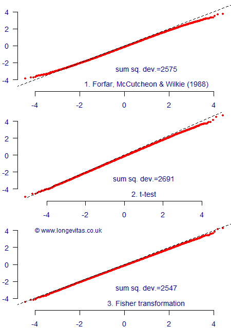
Figure 1 shows that all three test statistics do a similar job, although visually it looks like the Fisher transform performs best; this is particularly the case in the tails of the distribution, i.e. outside (-3, +3). We can quantify this performance by calculating the sum of squared deviations, i.e.

\[{\rm sum\ sq.\ dev.}=\sum_{j=1}^m (Z_j-Q_j)^2\]

where \(Z_j\) is the \(j^{\rm th}\) ordered test statistic, \(j=1,2,\ldots,m\) and where \(Q_j\) is the equivalent quantile of the theoretical distribution, i.e. N(0,1) for Forfar et al (1988) and the Fisher transform and the t-distribution for the other. In Figure 1 we have \(m=100,000\) and the sums of squared deviations have been added to the plots. We can see that our eyes have not deceived us — the Fisher transform has the lowest sum of squared deviations and thus its behaviour is the closest of the three to its theoretical distribution.

References:

Forfar, D. O., McCutcheon, J. J. and Wilkie, A. D (1988) On graduation by mathematical formula, Journal of the Institute of Actuaries, 115, 1–149.
Add new comment