A momentary diversion

An important quantity in mathematical statistics is the moment of a distribution, i.e. the expected value of a given power of the observations. Moments can be either raw, centred about a particular value or standardised in some way. The simplest example is the mean of a distribution: this is the raw first moment, i.e. the expected value of each observation raised to the power 1:

\[\mu = {\rm E}[X] = \int_{-\infty}^{\infty}xf(x)dx\]

The next example is the variance of a distribution: this is the second central moment, i.e. the expected value of the second power of the difference between each observation and the mean:

\[\sigma^2 = {\rm Var}[X] = \int_{-\infty}^{\infty}(x-\mu)^2f(x)dx\]

Other central moments can be defined similarly, e.g. for third and fourth central moments. In practice statisticians will often standardise moments, e.g. the standard deviation is the square root of the variance defined above. Similarly, rather than use the third and fourth central moments directly, statisticians will use standardised alternatives, such as skewness (third standardised moment) and kurtosis (fourth standardised moment).

Actuaries often have to perform simulations to investigate the nature of a risk, which involves summarising the main features of the underlying distribution. An important question is how big a sample size has to be to reliably measure these features? We can investigate this by calculating the moments for varying sample sizes of a known distribution. This is done in Figure 1 for simulated values from the N(0,1) distribution. The mean and standard deviation are therefore known to be zero and one, respectively, while the kurtosis is known to be 3 (the skewness of the Normal distribution is zero, so it is not shown to avoid confusion with the line for the mean).

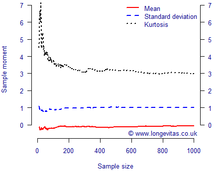
Figure 1 shows that a sample size of 100 is enough to fairly reliably estimate the mean and the standard deviation if the underlying distribution is Normal; there is relatively little additional accuracy to be gained for these moments with sample sizes above 200. However, even 200 observations is not enough to reliably estimate the coefficient of kurtosis, as the sample figure is still some distance away from its known theoretical value of 3. This is of interest to actuaries concerned with "1 in 200"-style measures, since kurtosis is a high-level measure of how much of the distribution lies in the tails; Figure 1 shows that hundreds of observations are required to assess the kurtosis, or "tailedness" of even a well-behaved distribution like N(0,1). In simulation work this can be addressed by increasing the number of simulations.

There is a flip-side to Figure 1, and that is model-fitting where the number of observations is fixed. For example, after the first fifty observations the mean is -0.17, the standard error is 0.79 and the kurtosis 4.19; these can be compared with the underlying known values of 0, 1 and 3. While the estimate of the mean is reasonable, the estimate of the standard deviation is over 20% too low. Furthermore, the coefficient of kurtosis would tempt many to conclude that the observations came from a distribution which had wider tails than the Normal distribution. However, as we can see from Figure 1, such a coefficient of kurtosis in a set of fifty N(0,1) variates is easily possible. This matters for time-series projection models, which are typically calibrated using the most recent fifty or so years of experience data and where an error term (the volatility) is commonly assumed to be Normally distributed. Unlike simulations, which can be increased in number at will, the calibration of projection models is limited to the data available. In addition to showing how many simulations are required to estimate features of a distribution, Figure 1 also shows how difficult it is to prove or disprove the assumption of Normality on the basis of a short time series.