Continuous improvement
In a previous blog I demonstrated that there was a statistically significant relationship between pension size and mortality. In a subsequent blog I looked at the improvements in model fit from treating pension size as a factor, but concluded that this was only a partial solution. In practice actuaries would prefer to avoid the discretisation error that comes with treating a real-valued variate as a discrete factor. Furthermore, it would be useful for pricing bases if a pension-size mortality effect could be extrapolated to values beyond those in the calibrating data set.
The first hurdle in modelling mortality continuously by pension size is the presence of extreme values in actuarial data sets. This is demonstrated for an English pension scheme in Figure 1(a).
Figure 1. Histograms of lives by pension size and some common transforms. Source: Richards (2020), ENG portfolio of lives in an English local-authority pension scheme.
![]()
Figure 1(a) demonstrates skewness, which can be partially addressed using some common transforms shown in panels (b) and (c). However, the real issue in Figure 1(a) is not skewness, but kurtosis, i.e. the extreme tail on the right due to some rare large pension values. The excess kurtosis of the pension values in Figure 1(a) is 19.1; for comparison, the equivalent figure for the Normal distribution is zero. Some of the other data sets in Richards (2020) have even more extreme excess kurtosis, so we cannot expect a simple transform like the logarithm or square root to address kurtosis across all data sets.
To flexibly address kurtosis we therefore use a parameterised transform function, \(\tau(s,\lambda_0)\), which maps the pension, \(s\), onto the interval \([0, 1]\). The parameter \(\lambda_0\) can then be varied to suit the level of kurtosis in the data set. Some candidate functions are shown in Figure 2 for \(\lambda=-10\); the precise details of the functions are available in Richards (2020).
Figure 2. Parameterised transform functions with \(\lambda_0=-10\). Source: Richards (2020).
![]()
The transform functions in Figure 2 are not only capable of adjusting to the kurtosis of the data set, but they are also capable of extrapolation: they all map a pension value \(s\in[0, \infty)\) onto \([0, 1]\) and are invertible. Once a transform function has been calibrated for a given value of \(\lambda_0\), it is possible to map any pension value. This not only means that we can interpolate between any pension values in the data set, but also that we can extrapolate beyond the uppermost value.
Having dealt with kurtosis via the transform function, the remaining step is to model mortality by the transformed pension value, \(u=\tau(s, \lambda_0)\). We do this by adding a life-specific pension-size effect, \(\alpha^{\rm amount}\), to log(mortality) as follows:
\[\alpha^{\rm amount}(u)=\omega^{\rm amount}(u)h_{01}(u)\qquad (1)\]
where \(h_{01}(u)\) is a cubic Hermite spline response function running from \(h_{01}(0)=0\) to \(h_{01}(1)=1\) and \(\omega^{\rm amount}\) represents the limiting adjustment to mortality (usually a reduction!) from having a practically infinite pension. Values of \(\lambda_0\) and \(\omega^{\rm amount}\) can be estimated from the data by optimising the log-likelihood, thus yielding a two-parameter model for mortality varying continuously by benefit size. Such a model has no discretisation error, and even permits extrapolation of a mortality basis to pension sizes outside the range of the calibrating data set. This is demonstrated in Figure 3, which shows the ratio of modelled mortality rates at various pension levels relative to the rates for those receiving £5,000 p.a.
Figure 3. Ratio of modelled mortality rates by pension size to those with £5,000 p.a. Source: Richards (2020).
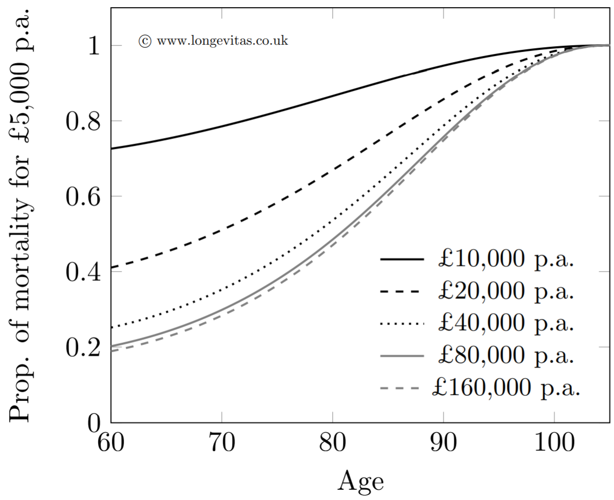
Figure 3 shows that large reductions in mortality at age 60 are possible from modest increases in pension size. As one might expect, further reductions become smaller as life's basic needs are increasingly met, with very little further reduction above £80,000 p.a. Of particular interest to actuaries looking to calibrate a pricing basis, the largest pension in the data set in Figure 3 was £103,000 p.a., but the approach outlined here has permitted a sensible extrapolation to be made for a pension of £160,000 p.a. courtesy of the transform function.
The continuous model requires just two parameters, yields smooth results without discretisation error and even produces extrapolations. But how does it compare to the discretised pension factors for the same portfolio? The answer is that the AIC for the model behind Figure 3 is 149,962, i.e. it is the same fit as the best-fitting, six-band model. In other words, we have just as good a fit, but without any of the drawbacks of discretisation error. Richards (2020) contains more details of the technical implementation of continuous amounts modelling, and gives results for portfolios from other countries.
References:
Richards, S. J. (2020) Modelling mortality by continuous benefit amount, Longevitas working paper.
Previous posts
Mortality patterns in time
The COVID-19 pandemic has created strong interest in mortality patterns in time, especially mortality shocks. Actuaries now have to consider the effect of such shocks in their portfolio data, and in this blog we consider a non-parametric method of doing this.
Add new comment