Frailty models

A population consists of individuals, each with their own genetics, lifestyle, and yes, their very own force of mortality. National mortality data, such as held by the Office for National Statistics (ONS), are observed only at the population level and the variation in the force of mortality across individuals of the same age is forever hidden. The purpose of this blog is to show how we can attempt to model this hidden heterogeneity.

Let us suppose that Gompertz really was right and that the mortality of each individual follows their own Gompertz law from ages 40 to 90, say. Notice that this is very different from saying that the mortality of the entire population (of individuals) follows the Gompertz law. Let us suppose that the force of mortality of an individual age \(x\) can be written as follows:

\[\mu_{x, z} = z \mu_x\qquad(1)\]

where \(\mu_x = \mu_{x,1}\) is the force of mortality for an individual with \(z=1\) and the factor \(z\) measures the departure of a particular individual from this standard.

If \(\mu_x\) follows the Gompertz law then equation (1) becomes:

\[\mu_{x, z} = z \exp(\alpha + \beta x) = \exp\{\log(z) + \alpha + \beta x\}\qquad(2)\]

and the force of mortality of the individuals in the population consists of parallel lines (on the log scale) (see Figure 2 below).

This idea goes back to the well-known actuary, Robert Beard (Beard, 1959), who referred to \(z\) as a 'longevity factor'. The paper by Vaupel, Manton and Stallard (1979) is better-known; they called the factor \(z\) the frailty of the individual. Clearly, if \(z=1\) we have a standard individual whereas \(z<1\) or \(z>1\) give individuals with relatively good or bad mortality respectively. Both these papers are required reading for those interested in mathematical models of mortality.

At this point both Beard and Vaupel et al assume that the distribution of the frailty \(z\) across the population follows a gamma distribution. For the purposes of this blog we will further assume that this distribution has mean 1 and standard deviation \(1/k\). Thus, the standard individual with \(z=1\) has the mean frailty.

Our model can be summarized as follows: the force of mortality of an individual age \(x\) with frailty \(z\), \(\mu_{x,z}\), can be written:

• \(\mu_{x,z} = z \mu_{x,1} = z \mu_x\)
• \(\mu_x = \exp(\alpha + \beta x)\)
• the pdf of \(z\) across the population is: \[f_Z(z) = {k^k \over \Gamma(k)} z^{k-1} e^{-kz},\; z > 0\qquad(3)\] the gamma distribution with mean 1 and variance \(1/k\).

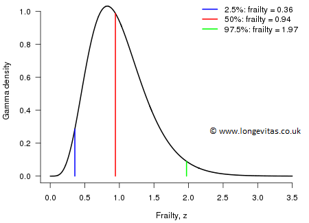
Figure 1 shows a typical frailty distribution, the gamma distribution with mean 1 and standard deviation 0.42; the median, the lower and the upper 2.5% frailty values are also shown. The force of mortality of the individuals in such a population varies widely: at the lower 2.5% point the individual has a force of mortality about one third of the standard while at the upper 2.5% the force of mortality is about twice that of the standard. These are large differences indeed.

Figure 1. Gamma frailty with mean 1 and standard deviation 0.42.

The question now is: what is the force of mortality \(h(x)\), say, that we observe at the population level? A simple if slightly tedious calculation shows that:

\[ h(x) = {e^{\alpha + \beta x} \over 1 + \displaystyle{{e^{\alpha + \beta x} - e^\alpha \over \beta k}}}\qquad(4)\]

A proof of this result is attached on the right for those interested. We can write equation (4) in the form:

\[ h(x) = {Be^{\beta x} \over 1 + De^{\beta x}}\qquad(5)\]

a form referred to by actuaries as a Perks curve after another well-known actuary, W Perks (1932). Some actuaries may be familiar with the alternative form:

\[ h(x) = {e^{{\alpha^\prime} + \beta x} \over 1 + e^{{\alpha^\prime} + \rho + \beta x}}\qquad(6)\]

where it is known as the Beard law of mortality (note that \(\alpha^\prime\) in equation (6) is different from \(\alpha\) in equation (4)); see Richards (2012) for a comprehensive list of these and other mortality laws. The technical note on the right contains a proof that the equations (4), (5) and (6) are equivalent.

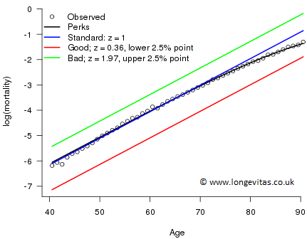
We illustrate these ideas with data on UK males in 1980 from ages 40 to 90 taken from the Human Mortality Database. We have the number of deaths \(d_x\) age \(x\) last birthday during 1980 and mid-year population estimates, the central exposures \(e_{x+1/2}\). We assume that \(D_x\), the random variable corresponding to the observed deaths \(d_x\), follows the Poisson distribution with mean \(e_{x+1/2}\mu_{x+1/2}\) and estimate by maximum likelihood. The frailty parameter \(k\) has estimated value 5.72 which gives a standard deviation of 0.42; this is the frailty distribution shown in Figure 1. Figure 2 shows the fitted Perks model; the fitted model fits the data rather well and picks up the slowing of the increase in the force of mortality at higher ages. The underlying individual forces of mortality are also shown for individuals with the median, the lower and the upper 2.5% frailties.

Figure 2: Log(mortality) for UK males in 1980 with fitted Perks population model, and fitted individual Gompertz models with frailties 1 (mean), 0.36 (lower 2.5% point) and 1.97 (upper 2.5% point).

The idea of a frailty model is conceptually attractive, but with population data we have no way of distinguishing between a population whose individuals either:

1. All follow a single Perks curve of mortality, or
2. Each have their own Gompertz curve of mortality that varies over the population with a gamma-distributed frailty.

Not distinguishing between these two, and mistakenly drawing conclusions about individuals based on group-level data, is known as the ecological fallacy. For my part, I favour the frailty model which chimes with my own view of individuals' life chances. Frailty models have many further interesting and sometimes surprising properties; we'll return to some of these at a later date.

References:

Beard, R. E. (1959). Note on some mathematical mortality models. In: Wolstenholme, G. E. W. and O'Conner, M. (eds.) The Lifespan of Animals. Ciba Foundation Colloquium on Ageing. Little, Brown, Boston, 302–311.
Human Mortality Database. University of California, Berkeley, USA. Available at www.mortality.org (data downloaded August, 2016).
Perks, W. (1932). On some experiments in the graduation of mortality statistics. Journal of the Institute of Actuaries, 63, 12–57.
R Core Team (2016). R: A Language and Environment for Statistical Computing. R Foundation for Statistical Computing, Vienna, Austria. URL https://www.R-project.org/.
Richards, S. J. (2012). A handbook of parametric survival models for actuarial use. Scandinavian Actuarial Journal, 2012, 233–257.
Vaupel, J. W., Manton, K. G. and Stallard, E. (1979). The impact of heterogeneity in individual frailty on the dynamics of mortality. Demography, 16, 439–454.
Add new comment