Over-dispersion (reprise for actuaries)
In my previous post I illustrated the effects of over-dispersion in population data. Of course, an actuary could quite properly ask: why use ONS data? The CMI data set on assured lives might be felt to be a better guide to the mortality of pensioners, although Stephen has raised a question mark over this assumption in the past.
Figure 1 illustrates what happens with the CMI data set. The over-dispersion parameter is much smaller at 1.82, so the Poisson model gives a reasonable forecast. Note that the over-dispersion in the CMI data comes from a different source, namely the presence of duplicates causing extra variability in death counts. However, the same approach to over-dispersion works regardless of the underlying cause of the extra variation.
Figure 1. Fitted and forecast values of log(mortality) at age 70 using different over-dispersion parameters. CMI data for male holders of life insurance policies.
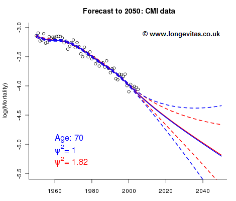
This story has a particularly happy ending for actuaries, since something very agreeable happens when we introduce over-dispersion into the forecasting procedure. As can be seen in Figure 1, the central forecast is scarcely changed, but the width of the confidence interval is much smaller. This is a general property of including over-dispersion in a Poisson model, and is a welcome piece of good news for the actuary demonstrating stress scenarios for ICA or Solvency II purposes!
Comments
Hi Iain,
Your posts on over-dispersion are very interesting. A good teaser to learn more. The finding in this analysis of CMI data, however, seems to me to be counter-intuitive from a stochastic point of view.
I have an inkling why overdispersion would improve your p-spline fit. However, if you were to do it "the other way round", i.e. assume that the process which gives rise to the data points is a stochastic process and project it forward using time series methods, your relaxation of the Poisson assumption leads to a widening of the confidence intervals, not a narrowing. Intuitively, my guess is that the overdispersion (or Negative Binomial assumption) increases parameter uncertainty, but for a given parameter set narrows the range of stochastic projections. In aggregate, however, the total range of outcomes should be substantially wider.
A comment on the other topic which your post touches on: ONS versus CMI.
I find it intuitively gratifying to see that CMI data is less dispersed than ONS data, which is as it should be, given the wider range of socio-economic strata in population data. However, again, parameter uncertainty in your stochastic model must be orders of magnitude greater for CMI data, because your ensemble is so much smaller. Again, this would lead to wider confidence intervals than the stochastic projection based on a best estimate parameter set implies.
Have you done any analysis on this issue?
BTW, you will have seen the ASTIN Bulletin (May 2009) article by Li, Hardy and Tan on overdispersion in mortality forecasts, won't you?
Greetings, Kai
Kai
I agree that the finding that the narrowing of the width of the confidence interval that results from the inclusion of over-dispersion in the smoothing process is "counter-intuitive from a stochastic point of view". The paradox is that what you say is absolutely correct but in the region of the data only The width of the confidence interval is indeed increased by a factor of about ψ=2.1 in the case of the ONS data and by a factor of about ψ=1.3 in the case of the CMI data - and the confidence interval does widen in the data region, just as we would expect. It is in the forecast region that the narrowing of the confidence interval occurs. In my blogs I just reported what happens and didn't discuss why this effect occurs. So something else is going on. Here are a couple of explanations.
With ONS data in particular we have large numbers of unacceptably large residuals under the Poisson assumption. The observed variation from a smooth curve is way in excess of what is reasonable under the Poisson distribution. What is the effect of these residuals on the smoothing process? The smoothing parameters must balance smoothness with fit. With very large residuals, fit wins at the expense of smoothness every time. The smoothing parameters will be set as small as possible since this optimizes with respect to fit, and essentially ignores smoothness. (Smoothness still remains but this is a consequence of the B-spline basis). But a fit with very small or zero smoothing parameters says there is a very weak signal into the future; alarmingly wide confidence intervals result.
Now let us introduce over-dispersion into the smoothing process (using the negative binomial distribution is an alternative way of introducing over-dispersion, as in Li, Hardy and Tan (ASTIN Bulletin, 2009)). Now the residuals are very much smaller and as a result the chosen curve does not have to go "chasing the data". The smooth curve can be chosen with (much) larger values of the smoothing parameters. Now we have a stronger signal; a narrower confidence interval in the forecast region results.
Here is a second, more technical explanation. The P-spline method has a Bayesian interpretation (see a famous paper by Brumback and Rice (1998) in the Journal of the American Statistical Association). Let θ be the regression coefficients, ie, the coefficients of the B-splines in the basis. Then the P-spline method is formally equivalent to assuming a normal prior distribution on θ with variance matrix equal to λ-1 M where M is a matrix which depends on the order of the penalty and λ is the smoothing parameter. Hence if λ is very small θ has a very large variance. As we go into the forecast region we rely more and more on the penalty and less and less on the data. But there is no information in the penalty - very wide confidence intervals result. With overdispersion, we have much larger values of the smoothing parameters, smaller variance on θ and everything behaves properly.
Far from being counter-intuitive, the widths of the confidence intervals behave exactly as they should when a smoothing method is employed.
Best wishes
Iain
Iain,
Many thanks for your explanations. As I said before, the findings are very interesting and your blog is a great motivation to study the p-splines approach in more detail.
Your work on over-dispersion I think is extremely important, because we are regularly faced with the problem of having to make the assumption of a "homogenous group" when analysing mortality experience, despite the fact that we know that the exposure is actually diverse in socio-economic, life-style (smoking habits) and other rating factors. Would you agree that introducing over-disperion is a powerful way of dealing with the inadequacy of our model, faced with lack of detailed, statistically credible data?
Thanks again and greetings from Cologne,
Kai
Kai
Two comments: (1) With aggregate data it seems it is the only tool we have. But (2) if you have your own (short-run) data with covariate information then you could think about a piggy-back model which will allow you to adjust forecasts from aggregate data in the light of your own dis-aggregated data.
Yours
Iain
Add new comment