Reducing uncertainty
The motto of the old UK Institute of Actuaries was certum ex incertis, i.e. certainty from uncertainty. I never particularly liked this motto — it implied that certainty can be obtained from uncertainty, whereas uncertainty is all-too-often overlooked. Fortunately, the merged Institute and Faculty of Actuaries picked a more sensible motto — e peritia ratio, i.e. reason from experience.
However, it is possible for uncertainty to be reduced, and one of the ways of doing this is with a properly constructed statistical model. For example, consider the mortality experience in a single year for a pension scheme where 32 deaths are observed in the age interval [75, 76) with 1,092.85 life-years of exposure. The estimated force of mortality at the middle of this age interval, \(\mu_{75.5}\), is then 0.029281 (being 32/1,092.85).
Of course, a point estimate is of little use without a statement of uncertainty, such as a confidence interval. In this example we can model the number of deaths in the group as following a Poisson distribution. As we saw in an earlier post, this assumption is technically not well specified as it allows for a non-zero probability of more deaths than lives under observation. However, the number of deaths here is large enough for this probability to be small enough to ignore this technical flaw in the group model. Using the Normal approximation to the Poisson distribution with mean and variance 32, we get a 95% confidence interval for the force of mortality of (0.019136, 0.039427). In general, mortality rates are often best expressed on a logarithmic scale — we will see why shortly — so our best estimate of \(\log\mu_{75.5}\) is -3.5308; the corresponding 95% interval is (-3.9562, -3.2333), i.e. the width of the 95% confidence interval is 20.5% of the estimate itself.
Now consider the plot of observed mortality rates at ages around age 75, as shown in Figure 1.
Figure 1. Crude mortality rates between ages 60 and 90 (logarithmic scale). Source: UK pension-scheme experience data for 2009 covering males and females.
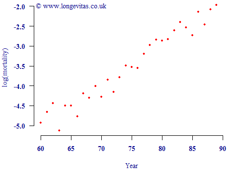
Apart from some random-looking volatility, it looks like mortality rates in Figure 1 are increasing in a straight line with age. This is the well-known Gompertz law of mortality:
\[\log\mu_x = \alpha+\beta x\]
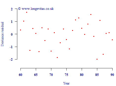
where \(x\) is age and \(\alpha\) & \(\beta\) are parameters to be estimated. Bearing in mind what we know about properly specifying models, we fit this model to the data for individual lifetimes, rather than the grouped counts (i.e. we fit an individual-level survival model). This gives us joint maximum-likelihood estimates for \((\alpha, \beta)\) of (-11.4089, 0.105373). We can check that this model is reasonable by examining the residuals, as shown in Figure 2. Since the residuals are a plausible scatter of N(0,1) variates, the model seems a good fit and soundly based.
Figure 2. Deviance residuals by age from fitting a Gompertz law to the data for the UK pension scheme in Figure 1.
Satisfied with the validity of the model, we return again to the question of estimating \(\log\mu_{75.5}\). Using our Gompertz model, the answer is -11.4089+0.105373*75.5 = -3.4532. This is different from the Poisson-based estimate, largely because our model has given us the opportunity to smooth out random variation. Furthermore, the Gompertz model also gives us a reduced error in estimating \(\log\mu_{75.5}\). The same procedure which gave us the maximum-likelihood estimates for α and β also gives us a variance-covariance matrix for those estimates. This tells us that Var(\(\alpha\))=0.108386, Var(\(\beta\))=1.75388x10⁻⁵ and Cov(\(\alpha, \beta\))=-0.00137207. Using the formula for the variance of correlated variables, we get an estimated variance of \(\log \mu_{75.5} =0.001178975\). This gives us a 95% confidence interval of (-3.5205, -3.3859), the width of which is only 3.9% of the estimate. This is a considerable improvement in the accuracy of estimation.
Why is the new estimate so much more accurate? The answer is because the Gompertz model for the force of mortality allows us to "borrow" information from adjacent ages. This also helps us to separate the underlying rate of mortality from the random variation, as shown in the plot of residuals in Figure 2. The residual plot tells us that the deviance residuals are plausibly from a N(0,1) distribution, and so the model seems valid, i.e. we really have reduced the uncertainty over the estimate. There are other business benefits of statistical models, but here the advantage lies in more accurate estimation of the underlying mortality rates.
Add new comment