Socio-economic differentials: convergence and divergence
Many western countries, including the UK, have recently experienced a slowdown in mortality improvements. This might lead to the conclusion that the age of increasing life expectancies is over. But is that the case for everyone? Or are there some groups in the UK who are still experiencing mortality improvements? The short answer is that mortality rates are still falling for the least deprived half of the population in England, while mortality improvements since 2011 have been virtually zero for the most deprived third. This has important consequences for reserving for pensions and annuities, so let us explore in a bit more detail. The findings in this blog are based on some early results of research carried out by Jie Wen, Andrew Cairns and me at Heriot-Watt University and the Actuarial Research Centre (ARC) of the Institute and Faculty of Actuaries.
The Office for National Statistics (ONS) recently released a data set with death counts, \(D_{x,y}\), and exposure data, \(E^c_{x,y}\), for England grouped by deprivation decile. The IMD (Index of Multiple Deprivation) measures the relative deprivation of people living in small areas in England; see ONS (2015). The ONS has ordered those areas by their IMD score, calculated the deciles (most deprived 10% to least deprived 10%) and published the mortality data for each decile for the years 2001–2015. We use these data to find out if there are differences in the level of mortality between IMD deciles (no surprise, there are differences), and more interestingly, differences between the improvement rates.
As we wish to consider an entire age range, rather than mortality rates at a specific age, we first fit a Lee-Carter model to each of the ten IMD deciles. As a reminder, the Lee-Carter model with death counts from a Poisson distribution is given by:
\[D_{x,y} \sim \mbox{Poisson}\big(m_{x,y} E^c_{x,y} \big) \mbox{ with } \log m_{x,y} = \alpha_x + \beta_x \kappa_y \]
where \(x = 40, \ldots, 89\) denotes age and \(y = 2001, \ldots, 2015\) denotes the calendar year. Fitting this model to each IMD decile separately we obtain the estimates for the age effects \(\alpha_x\) and \(\beta_x\) as shown in Figures 1 and 2:
Figure 1. Age effects, \(\alpha_x\), by IMD decile. Source: own calculations using ONS data.
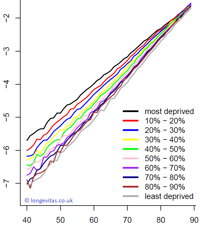
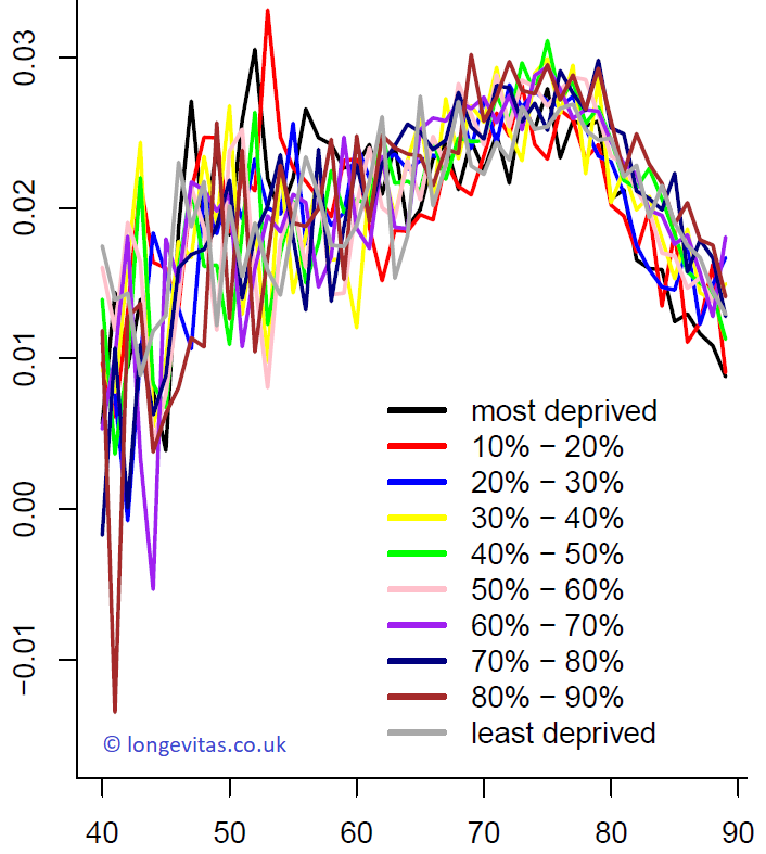
The plot of \(\alpha_x\) in Figure 1 can be interpreted as a baseline mortality rate for each individual age. As expected, there are substantial differences between mortality rates of the least deprived and the most deprived areas in England. What we also find is that at younger ages, the order of mortality rates follows almost exactly the order of IMD deciles. However, differences narrow with increasing age, a phenomenon known variously as mortality convergence or the compensation law of mortality. The second age effect, \(\beta_x\), is interpreted as an age-specific scaling of the period effect; in contrast to \(\alpha_x\), Figure 2 shows that \(\beta_x\) doesn't vary significantly between IMD deciles.
Figure 2. Age effects, \(\beta_x\), by IMD decile. Source: own calculations using ONS data.
While the level of mortality is captured by the leading age effects, \(\alpha_x\), the period effects \(\kappa_y\) show mortality improvements over time. Regular readers of this blog will know that the Lee-Carter model suffers from identifiability issues and that constraints need to be imposed on the parameters to obtain unique estimates. In particular, the level of the period effects \(\kappa\) cannot be uniquely determined. As we are interested in mortality improvements as captured by the drift of the period effect, we have imposed the constraint that the period effects start at zero for every IMD decile individually. As a consequence our baseline mortality \(\alpha_x\) corresponds to the fitted mortality rates in 2001, the first year in our data set.
Mortality improvements over time given by \(\kappa_y - \kappa_{y-1}\) can be uniquely identified in the Lee-Carter model (up to the scaling applied by the \(\beta_x\) term). We find in Figure 1 that the \(\beta_x\) for different IMD deciles are all similar and none dominates the others. In other words, changing the constraints will change the improvements observed in the period effect by a constant factor, but comparing those improvements between groups is still justified as long as the \(\beta_x\) terms are similar for all IMD deciles.
Figure 3. Period effects, \(\kappa_y\) for IMD deciles. Source: own calculations using ONS data.
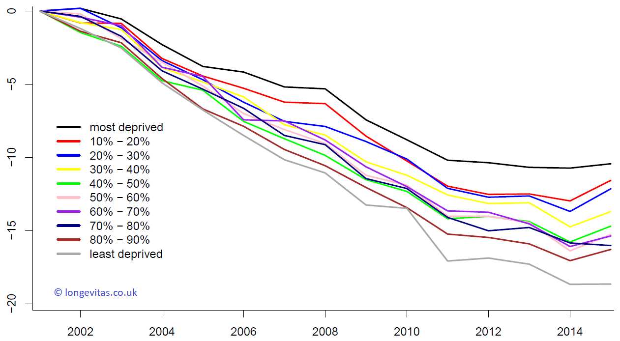
The period effects for our data are shown in Figure 3. We see that improvements are also different for the different groups. While the order is not so clear as it is for \(\alpha_x\), Figure 3 shows that the most deprived areas in England have experienced the smallest mortality improvements, while the least deprived have experienced the largest improvements. This has led to a widening gap in mortality by socio-economic group.
Now, have mortality improvements slowed down? Yes, this is our conclusion from Figure 3. But, more crucially, have improvements stopped? Well, that depends. To give a detailed answer we can calculate improvement rates for each IMD decile over different time horizons; see Table 1. We find that improvements are very different for the different groups.
Table 1. Estimated drift per annum of the period effects, \(\kappa_y\), by IMD decile and observation period. Source: own calculations using ONS data and model behind Figures 1–3.
| IMD decile | 2001– 2015 | Up to 2011 | From 2011 |
|---|---|---|---|
| most deprived | -0.75 | -1.02 | -0.06 |
| 10–20% | -0.83 | -1.20 | 0.10 |
| 20–30% | -0.87 | -1.21 | -0.01 |
| 30–40% | -0.98 | -1.26 | -0.28 |
| 40–50% | -1.05 | -1.42 | -0.13 |
| 50-60% | -1.09 | -1.40 | -0.31 |
| 60–70% | -1.10 | -1.37 | -0.43 |
| 70-80% | -1.14 | -1.41 | -0.48 |
| 80–90% | -1.16 | -1.52 | -0.26 |
| least deprived | -1.33 | -1.71 | -0.39 |
In particular, it seems that improvements have almost stopped since 2011 for about a third of the population of England, corresponding roughly to the 30% most deprived areas; see also Gavin's blog on occupational differentials. In contrast, for the least deprived 50% of the population in England we find that improvements have only slowed down, but clearly have not stopped. As mentioned above, changing the constraints changes our estimates in Table 1, but this does not affect our conclusion. Making improvement rates more comparable would require the use of a different model. This is the topic of some ongoing research at the ARC.
Why is all this important? People in less deprived areas are more likely to have pensions and annuities. They are also more likely to have larger pensions, a phenomenon known as concentration risk; see Richards (2008). It therefore seems advisable for annuity providers to continue to calculate reserves assuming some mortality improvement in future years. This becomes even more crucial when we take into account the rather short time period over which we have observed a slow down in improvements, just five years 2011–2015. The standard deviation of the estimate of the drift term of \(\kappa\) (not shown) is therefore relatively large. For projections based on random-walk models this parameter uncertainty will be more important than volatility beyond a horizon of five years; see Kleinow & Richards (2016).
To conclude: socio-economic differentials in mortality are clear, but reduce with age. However, these differentials have widened over time and continue to do so. Pension schemes and annuity portfolios therefore need to be careful when using projections calibrated to mortality data from the entire population. The near-zero improvements amongst the most deprived third of the population are masking the stronger improvements of the least deprived, i.e. the ones who account for a disproportionate share of pension-scheme liabilities. The use of all-population data to calibrate projection models when liabilities are concentrated in a sub-group is a form of basis risk, against which insurers are expected to hold extra reserves.
References:
Kleinow, T. and Richards, S. J. (2016) Parameter risk in time-series mortality forecasts, Scandinavian Actuarial Journal, 2016(10), pages 1–25.
Office for National Statistics (2015) English indices of deprivation 2015, Ministry of Housing, Communities & Local Government.
Richards, S. J. (2008), Applying survival models to pensioner mortality data, British Actuarial Journal, 14(II), pages 257–326 (with discussion).

Add new comment