Valuing liabilities with survival models
Regular readers of this blog will know that we are strong advocates of the benefits of modelling mortality in continuous time via survival models. What is less widely appreciated is that a great many financial liabilities can be valued with just two curves, each entirely determined by the force of mortality, \(\mu_{x+t}\), and a discount function, \(v^t\).
The first of these useful curves is the discounted survival function, \({}_tp_xv^t\), where \({}_tp_x\) is the probability of survival from age \(x\) to age \(x+t\). If you know the force of mortality, then you know the survival probability from the following fundamental relationship:
\[{}_tp_x=\exp\left(-\int_0^t\mu_{x+s}ds\right).\]
For a derivation of the above, see my earlier blog. The discount function, \(v^t\), can be based on either a constant interest rate or else a more flexible yield curve. An example discounted survival function based on the Gompertz force of mortality, \(\mu_x=e^{\alpha+\beta x}\), is shown in Figure 1.
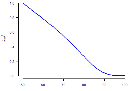
There are several liabilities we can value using the discounted survival function in Figure 1:
- Pure endowment. Here the payment is only made on survival to age \(x+n\), so we simply read off the value for \({}_np_xv^n\).
- Lifetime annuity in payment. Here the payment is made as long as the life is alive, so we integrate \({}_tp_xv^t\) over \(t\in[0, \infty)\).
- Deferred annuity. Here the payment is made as long as the life is alive after age \(x+n\), so we integrate \({}_tp_xv^t\) over \(t\in[n, \infty)\).
- Temporary annuity. Here the payment is made as long as the life is younger than age \(x+n\), so we integrate \({}_tp_xv^t\) over \(t\in[0, n)\).
That is four different product types that we can value using the discounted survival function. The other useful curve is the discounted curve of deaths, \({}_tp_x\mu_{x+t}v^t\), an example of which is plotted in Figure 2.
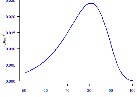
The discounted curve of deaths in Figure 2 has application in valuing assurances:
- Whole-of-life assurance. This pays out on death at any future age, so we integrate \({}_tp_x\mu_{x+t}v^t\) over \(t\in[0, \infty)\).
- Term assurance. This pays out on death before age \(x+n\), so we integrate \({}_tp_x\mu_{x+t}v^t\) over \(t\in[0, n)\).
There is another product which can be valued using a combination of Figures 1 and 2:
- Endowment assurance. This pays out on death before age \(x+n\), or on surviving to age \(x+n\). This is a combination of a term assurance and a pure endowment, so we integrate \({}_tp_x\mu_{x+t}v^t\) over \(t\in[0, n)\) and add \({}_np_xv^n\).
That is seven basic product types that can be valued using the two functions. Other products can be valued too — for example, a bridging pension for a not-yet-retired pension-scheme member is a deferred temporary annuity between scheme retirement age, \(x_1\), and state pension age, \(x_2\); for \(x<x_1<x_2\) this would be valued by integrating \({}_tp_xv^t\) over \(t\in[x_1-x, x_2-x)\).
One remaining question is how best to integrate under these curves. It is rare to have closed-form expressions, so one of two approaches is typically used:
- If you have an explicit functional form for \({}_tp_x\) that you can evaluate for any \(x\) or \(t\), you can use a function like \(\tt integrate()\) in R.
- If you only have \({}_tp_x\) and \(\mu_{x+t}\) for specific values of \(x\) and \(t\), say at intervals of one year, then you can use numerical integration over a grid of fixed points.
In both cases the approximations are fast and accurate. Our recently published book, Modelling Mortality with Actuarial Applications, gives sample R code and explores the level of accuracy achievable under each approach in Appendix D.
References:
Macdonald, A. S., Richards, S. J. and Currie, I. D. (2018) Modelling Mortality with Actuarial Applications, Cambridge University Press., pages 344–346.
Add new comment