Longevity capital requirements on the edge
in Kleinow & Richards (2016, Table 5) we noted a seeming conundrum: the best-fitting ARIMA model for the time index in a Lee-Carter model also produced much higher value-at-risk (VaR) capital requirements for longevity trend risk. How could this be?
We first note that the best-fitting model was chosen with reference to the AIC with the small-sample correction factor. Thus, the model had the best fit (i.e. highest log-likelihood) while balancing the complexity of the model (i.e. taking into account the parameter count and the small sample size). So how could the best-fitting model produce the highest capital requirement? In Kleinow & Richards (2016) we used a bootstrapping procedure from Pascual et al (2004) to examine the densities of the parameter estimates, as shown in Figure 1:
Figure 1. Estimated densities of autoregressive (AR) and moving-average (MA) parameters in ARIMA(1,1,2) model fitted to time index in Lee-Carter model fitted to males in England & Wales, ages 50-104 over the period 1971-2013. Source: Kleinow & Richards (2016, Figure 5).
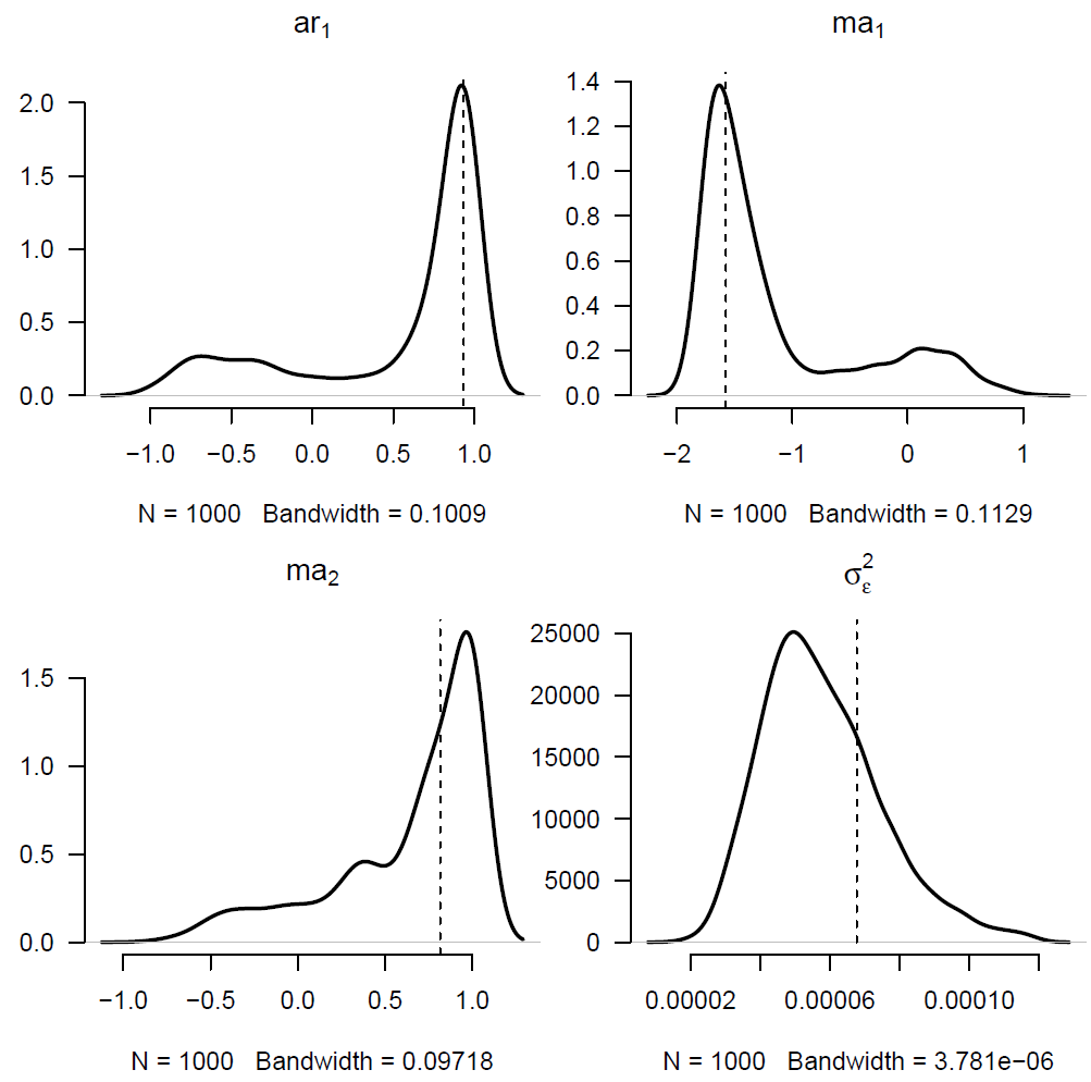
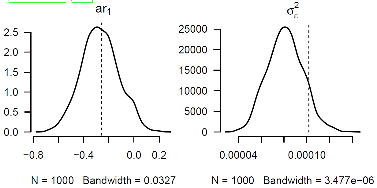
Strictly speaking these are dependent parameters, so we should present a joint density in four dimensions. However, Figure 1 shows that the densities are highly skewed, so the addition of new data can make material changes to the parameter estimates. The autoregressive parameter dictates the behaviour of the forecast, and so a large shift in the value of the ar1 parameter will produce a large change in the forecast. This is the underlying reason why this particular ARIMA(1,1,2) model leads to higher capital requirements than simpler ARIMA models. By way of contrast, Figure 2 shows the estimated parameter densities for a simpler ARIMA(1,1,0) model with lower VaR capital requirements:
Figure 2. Estimated densities of autoregressive (AR) parameter in ARIMA(1,1,0) model fitted to time index in Lee-Carter model fitted to males in England & Wales, ages 50-104 over the period 1971-2013. Source: Kleinow & Richards (2016, Figure 8).
Can we detect the potential instability behind Figure 1 without all the time-consuming bootstrapping simulations and model refits? One possibility might be an examination of the roots of the characteristic equation of an ARIMA model. Without reprising the mathematics, there are two parts:
The roots for the autoregressive (AR) part of the ARIMA model, and
The roots for the moving-average (MA) part of the ARIMA model.
In general the roots will be complex numbers. A stationary ARIMA model will have all its roots outside the unit circle. However, it is easier to plot and check if values lie inside the unit circle, so we typically plot the inverse roots (which will also be complex numbers in general). Figure 3 plots the inverse roots for the best-fitting ARIMA(1,1,2) model in Kleinow & Richards (2016, Table 3).
Figure 3. Inverse roots of the characteristic polynomials for the ARIMA(1,1,2) model in Kleinow & Richards (2016, Table 3). Source: own calculations using data for males aged 50-104 in England & Wales over the period 1971-2013.
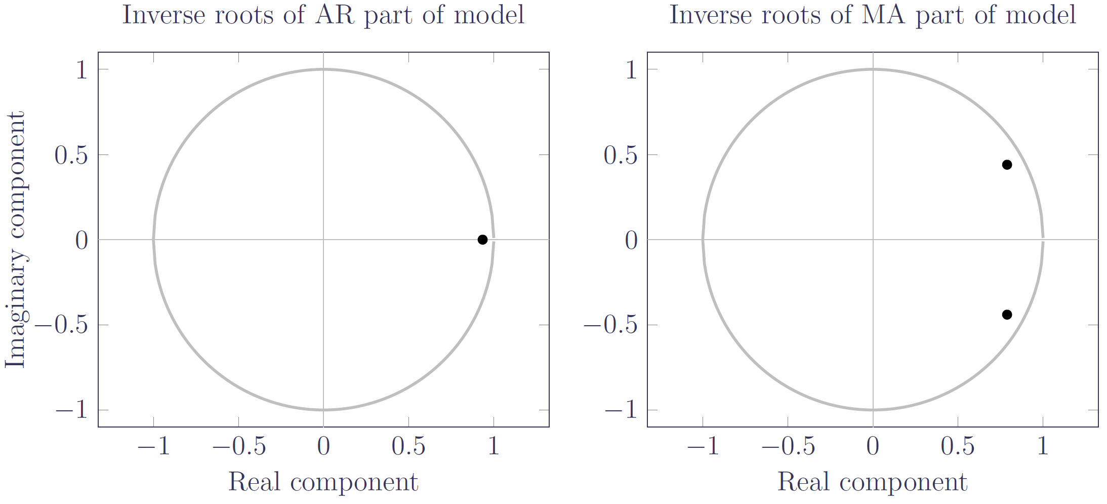
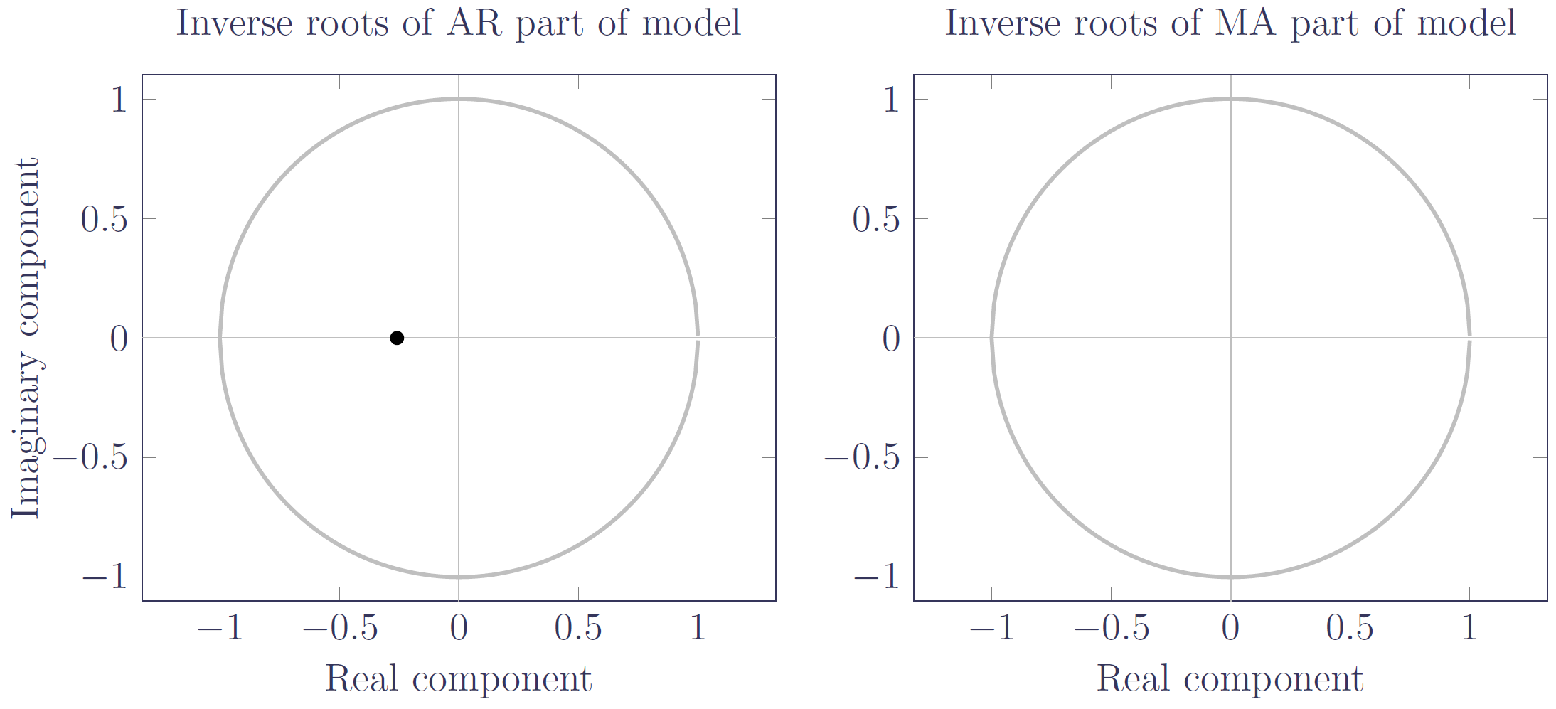
Figure 3 shows that the inverse roots lie within the unit circle, as one would expect for a stationary model. However, the roots are rather close to the unit circle, suggesting that the model could be easily perturbed to a different state. In contrast, the inverse root for the ARIMA(1,1,0) model in Figure 4 is far from the edge, and the model unsurprisingly produces less variable forecasts in a value-at-risk assessment:
Figure 4. Inverse root of the characteristic AR polynomial for the ARIMA(1,1,0) model in Kleinow & Richards (2016, Table 3); there are no MA roots. Source: own calculations using data for males aged 50-104 in England & Wales over the period 1971-2013.
Forecast stability is a desirable property of a stochastic mortality model, although not at any price. One option might be to not always pick the best-fitting ARIMA model, especially if there is a closely-placed alternative candidate with better properties. However, in the case of Kleinow & Richards (2016, Table 2) the five ARIMA models with the lowest AICc all had inverse roots close to unit circle like Figure 3. Clearly there is something about this particular Lee-Carter time index that drives more variable ARIMA forecasts, thus leading to higher VaR capital requirements.
References:
Kleinow, T. and Richards, S. J. (2016) Parameter risk in time-series mortality forecasts, Scandinavian Actuarial Journal, 2016(10), pages 1-25, doi:10.1080/03461238.2016.1255655 (preprint available).
Pascual, L., Romo, J. and Ruiz, E. (2004) Bootstrap predictive inference for ARIMA processes, Journal of Time Series Analysis, 25(4), pages 449-465, doi:10.1111/j.1467-9892.2004.01713.x.
Richards, S. J., Currie, I. D. and Ritchie, G. P. (2014) A value-at-risk framework for longevity trend risk, British Actuarial Journal, 19(1), pages 116-167, doi 10.1017/S1357321712000451 (preprint and supporting materials available).
ARIMA roots in the Projections Toolkit
The inverse roots of ARIMA characteristic polynomials appear in the PDF report from v2.8.7.
Add new comment