Modelling mortality shocks

The ongoing coronavirus pandemic has so far produced two mortality shocks in the UK and many other countries.  Unsurprisingly, the extra mortality is also visible in annuity portfolios.  Such mortality spikes create a challenge for actuaries — how do you model a portfolio's mortality experience when the period covered includes one or more pandemic shocks?

Actuaries analyse recent experience data to set a best-estimate basis (future trends or improvements are usually handled as a separate basis item).  However, the presence of a mortality shock creates a risk of upward bias (unless you want to assume that such mortality shocks will regularly re-occur).  One thought might be to remove all deaths with covid-19 on the death certificate.  However, I have yet to encounter a pension scheme or annuity portfolio that records the cause of death, so this cannot be a general solution.  Another thought might be to ignore the main periods of covid-affected mortality.  However, this carries two drawbacks.  The first is that pension schemes in particular often only have 3–5 years of experience data, so discarding some of that data is an unaffordable luxury when pricing a longevity swap.  The second drawback is that the mortality shocks occur at focused points in the year.  Since mortality has a pronounced seasonal pattern, ignoring periods of pandemic mortality would lead to balanced seasons.  This would create a new source of bias to replace the bias we were trying to eliminate in the first place.

A better idea would be to use all the available data, but for the mortality model to handle sharp fluctuations in time. It is essential that the model doesn't require any new data fields beyond what is usually available in administration systems. One approach is the following model for the mortality hazard, \(\mu_{x,y}\), at age \(x\) and calendar time \(y\):

\[\log \mu_{x,y} = \log \mu_x + \displaystyle\sum_{j\ge 1} \kappa_{0,j} B_j(y)\qquad (1)\]

where:

• \(\mu_x\) is the age-varying mortality hazard, including covariates like gender and annuity amount,
• \(B_j(y)\) is the \(j^{\rm th}\) \(B\)-spline evaluated at \(y\), and
• \(\kappa_{0,j}\) is the coefficient of \(B_j\).

Figure 1 shows an example \(B\)-spline basis with a one-year gap between knot points.

Figure 1. A basis of nine equally spaced splines spanning 1st January 2015 to end-2020; splines are numbered \(j=0,\ldots,8\). Source: Richards (2021, Figure 12).

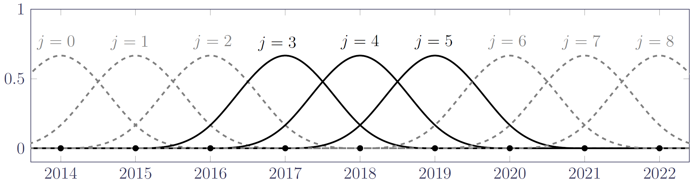
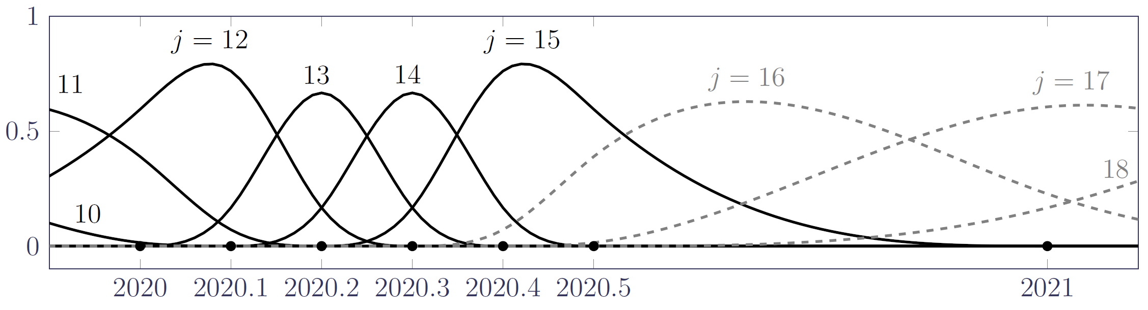
However, we obviously need closer knot spacing for modelling shocks that take place over a couple of months. We further note that there is no requirement for knot points to be equally spaced. This means that we can add knots only where greater flexibility is needed, e.g. around the time of a mortality shock. Figure 2 shows part of an alternative basis of \(B\)-splines with a half-year gap between knots (to capture seasonal variation), plus additional knots around the time of the first covid-19 shock in the UK in April and May 2020.

Figure 2. Excerpt from a basis of nineteen variably spaced splines spanning 1st January 2015 to end-2020; only splines \(j=10,\ldots,18\) are shown. Source: Richards (2021, Figure 16).

The model in equation (1) fits a continuous age-period model, meaning that the time component of mortality is independent of age (although the estimates of \(\kappa_{0,j}\) are obviously influenced by the age range of the data used to calibrate the model). Figure 3 shows the results of fitting the model in equation (1) to a portfolio of UK annuitants, where \(\mu_x\) accounts for mortality by age, gender and annuity amount:

Figure 3. Age-independent pattern of mortality in time for UK annuity portfolio. The function plotted is \(\exp\left(\sum_{j\ge 0}(\hat\kappa_{0,j}-c_{2019.75})B_j(y)\right)\), where \(c_{2019.75}\) is a normalising constant so that the function takes the value 1 at 1st October 2019. Source: Richards (2021, Figure 17b).

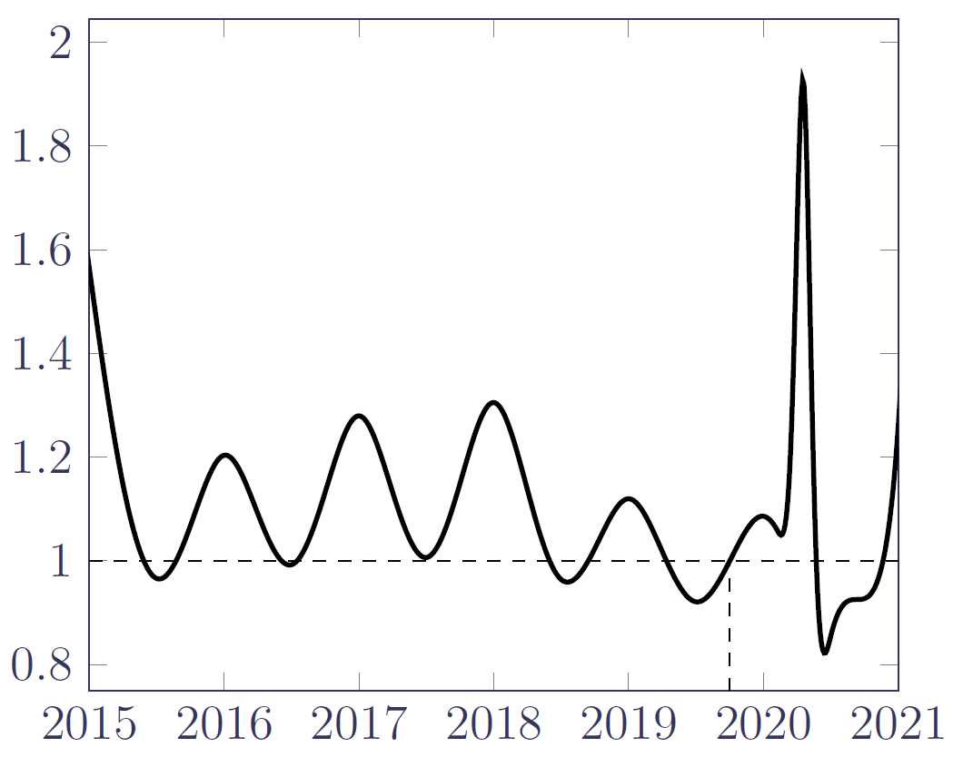
For analysis purposes we set a reference mortality level of 1 mid-way between the summer trough of 2019 and the winter peak of January 2020; this doesn't change the fitted model, but it does aid interpretation. Figure 3 shows that the model in equation (1) is capable of identifying a rich variety of mortality patterns in time, including the seasonal variation over 2015–2019 and the first covid-19 mortality shock of April & May 2020. The most striking aspect is the doubling of the mortality hazard during the mortality shock compared to the reference level. Another feature is the extent of the trough-to-peak seasonal variation, with winter mortality levels up to 30% higher than summer mortality dips. A third aspect is the suggestion of an unusually deep summer trough in 2020; this could be a result of brought-forward deaths of the frail in the mortality shock ("harvesting"), or else a result of healthier behaviours of a socially distanced population under lockdown (or perhaps both).

The usefulness of Figure 3 to the actuary is evident: with a clear picture of mortality levels in continuous time, she can be sure that the other parameters in the model are not biased by mortality shocks or seasonal variation. Setting a best-estimate basis is then a question of deciding what time-point represents a suitable level for the purpose at hand, such as setting a pricing basis for a bulk annuity or a longevity swap. This is a matter of actuarial judgement, but one which will be informed by the detailed insights from Figure 3.

References:

Richards, S. J. (2022) Allowing for shocks in portfolio mortality models, British Actuarial Journal, 2022;27:e1, doi:10.1017/S1357321721000180.
Add new comment