The Hermite model of mortality
In Richards (2012) I compared seventeen different parametric models for modelling the mortality of a portfolio of UK annuitants. The best-fitting model, i.e. the one with the lowest AIC, was the Makeham-Beard model:
\[\mu_x = \frac{e^\epsilon+e^{\alpha+\beta x}}{1+e^{\alpha+\rho+\beta x}}\qquad(1)\]
where \(\mu_x\) is the force of mortality at age \(x\) and \(\alpha\), \(\beta\), \(\epsilon\) and \(\rho\) are parameters to be estimated. These parameters have interpretations, e.g. \(\beta\) is broadly the rate at which the force of mortality increases by age on a logarithmic scale, \(e^\epsilon\) is the constant background rate of mortality and \(e^{-\rho}\) is the limiting force of mortality as \(x\to\infty\) (if \(\beta>0\), as is invariably the case). The Makeham-Beard model arises in a number of different ways, for example as the limit of the cascade model of mortality.
An alternative is to use non-parametric methods, such as the Kaplan-Meier survival function. Non-parametric methods do not have parameters to interpret, and nor can they provide extrapolated rates beyond the available data. Despite this, they can be very useful for checking data quality and communicating with non-technical audiences.
Between non-parametric and parametric models lies a third group: pseudo-parametric models. As with parametric models there are parameters to be estimated, but they often do not have simple real-world interpretations like parametric models (although one must always be careful in this regard, especially with projection models). One of the commonest forms of pseudo-parametric model involves splines, of which there are many different kinds and representations. Much of Iain Currie's work involves \(P\)-splines, for example, although there is a veritable menagerie in this field: from Bézier curves to thin-plate splines. What connects all these methods is the idea of using a set of overlapping basis functions to provide both flexibility and smoothness.
One option is to use cubic Hermite splines, which are widely used in computer graphics for tracing a smooth path between two points, A basis for cubic Hermite splines is shown in Figure 1:
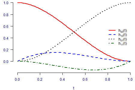
Sticking with the computer-graphic metaphor, we imagine that we want to trace a smooth curve between the mortality rate at the youngest age, \(x_0\), to the oldest age, \(x_1\). We might set \(x_0=50\) and \(x_1=120\), say, although we will often want to extrapolate values outside this range. We can therefore define our force of mortality as a linear combination of the Hermite functions as follows:
\[\log\mu_x =\begin{cases}x\le x_0&: \alpha\\x_0\lt x\lt x_1&: h_{00}(t)\alpha + h_{01}(t)\omega + h_{10}(t)m_0+h_{11}(t)m_1\\x\ge x_1&: \omega\end{cases}\qquad(2)\]
where \(t=(x-x_0)/(x_1-x_0)\) and \(h_{00}\), \(h_{10}\), \(h_{01}\) and \(h_{11}\) are the Hermite basis functions depicted in Figure 1. As it happens, \(\alpha\) then represents \(\log\mu_{x_0}\) and \(\omega\) represents \(\log\mu_{x_1}\), i.e. the log force of mortality at the youngest and oldest ages, respectlvely. We are therefore tracing a smooth curve between the points \((x_0, \alpha)\) and \((x_1, \omega)\). \(m_0\) is the initial gradient of the curve as it leaves \((x_0, \alpha)\), while \(m_1\) is the gradient of the curve as it approaches \((x_1, \omega)\). This is depicted in Figure 2.
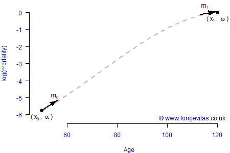
Although we have presented things graphically in Figure 2, the parameters \(\alpha\), \(\omega\), \(m_0\) and \(m_1\) can be estimated in a survival model. The results of doing so for a UK local-authority pension scheme are shown in Table 1, and the fit is shown in Figure 3.
Table 1. Estimates of parameters in full Hermite model. Source: own calculations using data from UK local-authority pension scheme, ages 60–100 observed 2000–2009.
| Parameter | Name | Estimate |
|---|---|---|
| \(\alpha\) | Intercept | -5.76319 |
| \(\omega\) | Oldest | 0.00764617 |
| \(m_0\) | AgeGradientStart | 5.82051 |
| \(m_1\) | AgeGradientEnd | 0.912123 |
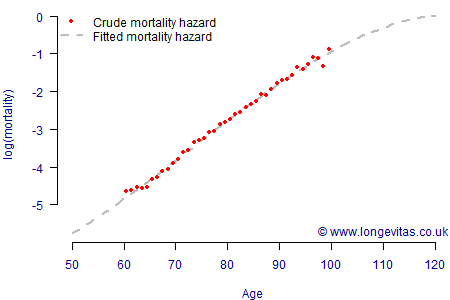
In addition to providing a good fit, Figure 3 shows that the Hermite model is also capable of sensible extrapolation outside the data range at either end, as with most parametric models. Although the Hermite parameters don't offer a term like the rate of ageing (\(\beta\) in equation (1)), they do have a simple interpretation that \(\alpha=\log\mu_{x_0}\) and \(\omega=\log\mu_{x_1}\). For full technical details of the model, see Richards (2019) or the interactive plotting tools here.
References:
Richards, S. J. (2012) A handbook of parametric survival models for actuarial use, Scandinavian Actuarial Journal, 2012(4), pages 233–257.
Richards, S. J. (2019) A Hermite-spline model of post-retirement mortality, Scandinavian Actuarial Journal (to appear).
Add new comment