The perils of parameter interpretation
With some notable exceptions, such as the Kaplan-Meier estimator, most mortality models contain parameters. In a statistical model these parameters need to be estimated, and it is a natural thing for people to want to place interpretations on those parameter estimates. However, this can be tricky, as parameters in a multi-parameter model are dependent on each other.
We will illustrate this with the Lee-Carter model, which is perhaps the most durable stochastic projection model in use today. It is structured as follows:
log μx,y = αx + βxκy (1)
where μx,y is the force of mortality at age x in year y, and αx, βx and κy are parameters to be estimated. The Lee-Carter model is widely used, including throughout our own articles, and some example values for β and κ are plotted in Figure 1.
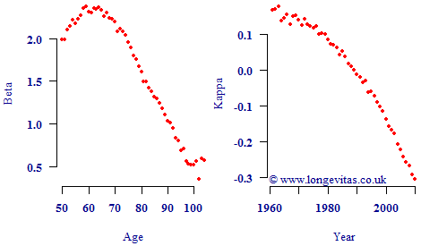
Looking at Figure 1 it is tempting to conclude that the κ process represents the overall level of mortality, as modulated by the age-related parameter β. However, now consider the parameter plots in Figure 2. Figure 2 looks a little strange because κ is rising over a period when we know mortality rates have been falling strongly, so how can κ represent the overall level of mortality? Nevertheless, these alternative values for β and κ produce the same maximum log-likelihood value, the same fitted values for log μ and result in the same projected values. Both sets of parameters also satisfy exactly the same constraints. There is therefore no mathematical or statistical reason to prefer the parameterisation in Figure 1 over that in Figure 2.
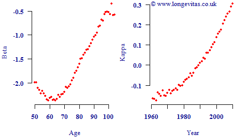
The reason for the two parameterisations being equivalent lies in the formulation of Equation (1) — if you switch the sign of both βx and κy, you get the same addition to αx. As it happens, we tend to prefer the parameterisation in Figure 1, but whether you get Figure 1 or Figure 2 depends on your initial values and your fitting algorithm.
In the case of the Lee-Carter model, it does not in fact matter which of the two parameterisations we use. Both will lead to the same fitted values and the same projections. However, this may not be true in more complex models, and this example serves to underline the danger of assuming parameter values have a particular meaning in isolation. This is particularly the case where there are both period- and cohort-based parameters involved in a model.
Add new comment