Normal behaviour

One interesting aspect of maximum-likelihood estimation is the common behaviour of estimators, regardless of the nature of the data and model.  Recall that the maximum-likelihood estimate, \(\hat\theta\), is the value of a parameter \(\theta\) that maximises the likelihood function, \(L(\theta)\), or the log-likelihood function, \(\ell(\theta)=\log L(\theta)\).  By way of example, consider the following three single-parameter distributions:

1. The number of events, \(D\), in a binomial(\(n\), \(q\)) distribution.

2. The number of events, \(D\), in a Poisson(\(E\mu\)) process, and

3. The sum, \(E\), of \(n\) observations from the exponential(\(\lambda\)) distribution.

The response variable \(D\) in (1) and (2) is a non-negative integer, while the response variable \(E\) in (3) is a positive real number.  The log-likelihood functions are as follows:

1. \(\ell(q|n, d) = (n-d)\log(1-q)+d\log q\)

2. \(\ell(\mu|E, d) = d\log\mu-E\mu\)

3. \(\ell(\lambda|n, E) = n\log \lambda-E\lambda\)

where the conventional notation is \(\ell({\rm parameter}|{\rm data})\).  The close parallel between the log-likelihoods in (2) and (3) is a reminder that the time between events in a Poisson process has an exponential distribution.  Although the three distributions are different, the log-likelihood functions have a similar shape around the MLE, as shown in Figure 1.

Figure 1.  Log-likelihood functions around maximum-likelihood estimates.  Source: own calculations using \(n=1000\) and \(d=200\) for the binomial distribution, \(d=200\) and \(E=900\) for the Poisson distribution and \(n=200\) and \(E=38.47979\) for the exponential distribution.

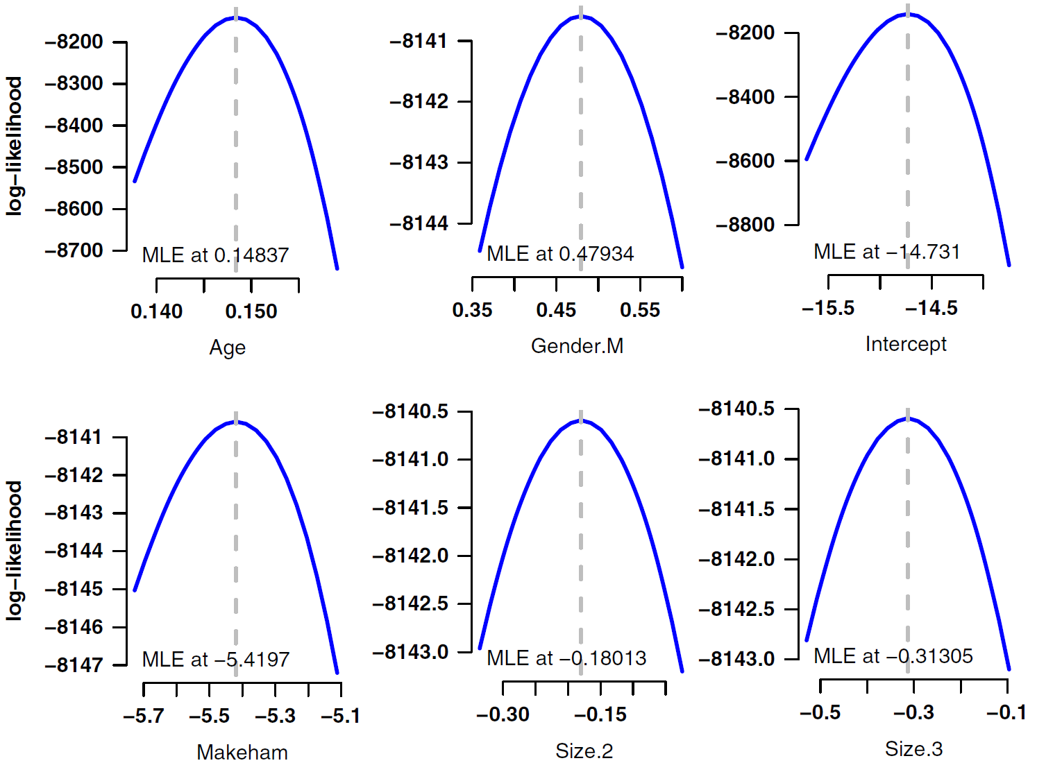
Figure 1 shows that, regardless of the model, the log-likelihood function has a quadratic shape around the maximum-likelihood estimate.  This is not an accident - the maximum-likelihood theorem says that the distribution of a maximum-likelihood estimator is normal (Gaussian) around the MLE.  This extends to multivariate models, where the joint maximum-likelihood estimator has a multivariate normal distribution with mean \(\boldsymbol{\theta}\) and covariance matrix \(\boldsymbol{\Sigma}\) (using bold type to signal vectors and matrices).  Multivariate likelihoods are trickier to plot, but one approach is to use profile likelihoods, i.e. varying each parameter in turn while holding the other parameters constant at their MLE.  Some examples are shown in Figure 2.

Figure 2.  Profile log-likelihoods for selected parameters from a multi-factor model of pensioner mortality.  Source: Richards (2016, page 445).

This is a very handy result for actuaries considering mis-estimation risk: whatever the model specification, joint MLEs have a multivariate normal distribution.  The vector mean of the distribution is estimated with \(\boldsymbol{\hat\theta}\), while the covariance matrix is estimated from the inverse of the observed information matrix.  We can then assess mis-estimation risk by valuing the liabilities using parameter vectors sampled from this multivariate normal distribution.  Richards (2016) presents a methodology for assessing mis-estimation risk in run-off, while Richards (2021) presents a methodology for calculating mis-estimation capital under a value-at-risk (VaR) regime.

References:

Richards, S. J. (2016) Mis-estimation risk: measurement and impact, British Actuarial Journal, 21(3), 429-457. doi 10.1017/S1357321716000040.
Richards, S. J. (2021) A value-at-risk approach to mis-estimation risk, British Actuarial Journal, 26, e13, pages 1–20, doi 10.1017/S1357321721000131.
Likelihoods and mis-estimation in Longevitas
Each model in Longevitas has a Parameters tab that allows the plotting of profile log-likelihoods.
Longevitas offers two types of mis-estimation assessment:
Run-off mis-estimation, i.e. where parameter risk applies across the lifetime of the liabilities being valued. This is appropriate to pricing the transfer of risk, such as with bulk annuities, longevity swaps and reinsurance.
Value-at-risk mis-estimation, i.e. the sensitivity of liabilities to recalibration risk. This is suitable for Solvency II-style capital assessment.
Users can switch between the two using the configuration option Mis-Estimation VaR Horizon.
Add new comment