Walking the Line

In mortality forecasting work we often deal with downward trends.  It is often tempting to jump to the assumption of a linear trend, in part because this makes for easier mathematics.  However, real-world phenomena are rarely purely linear, and the late Iain Currie advocated linear adjustment as means of judging linear-seeming patterns.  This involves calculating a line between the first and last points, and deducting the line value at each data point to reveal the local behaviour.  A random-seeming scatter about zero will indicate a linear relationship, but correlated deviations will indicate something more complex.  In this blog we will explore how random walks and (especially) ARIMA models provide good representations of not-quite-linear mortality trends.

By way of example, consider the Lee-Carter model for mortality at age \(x\) in year \(y\):

\[\log\mu_{x,y} = \alpha_x + \beta_x\kappa_y\qquad(1)\]

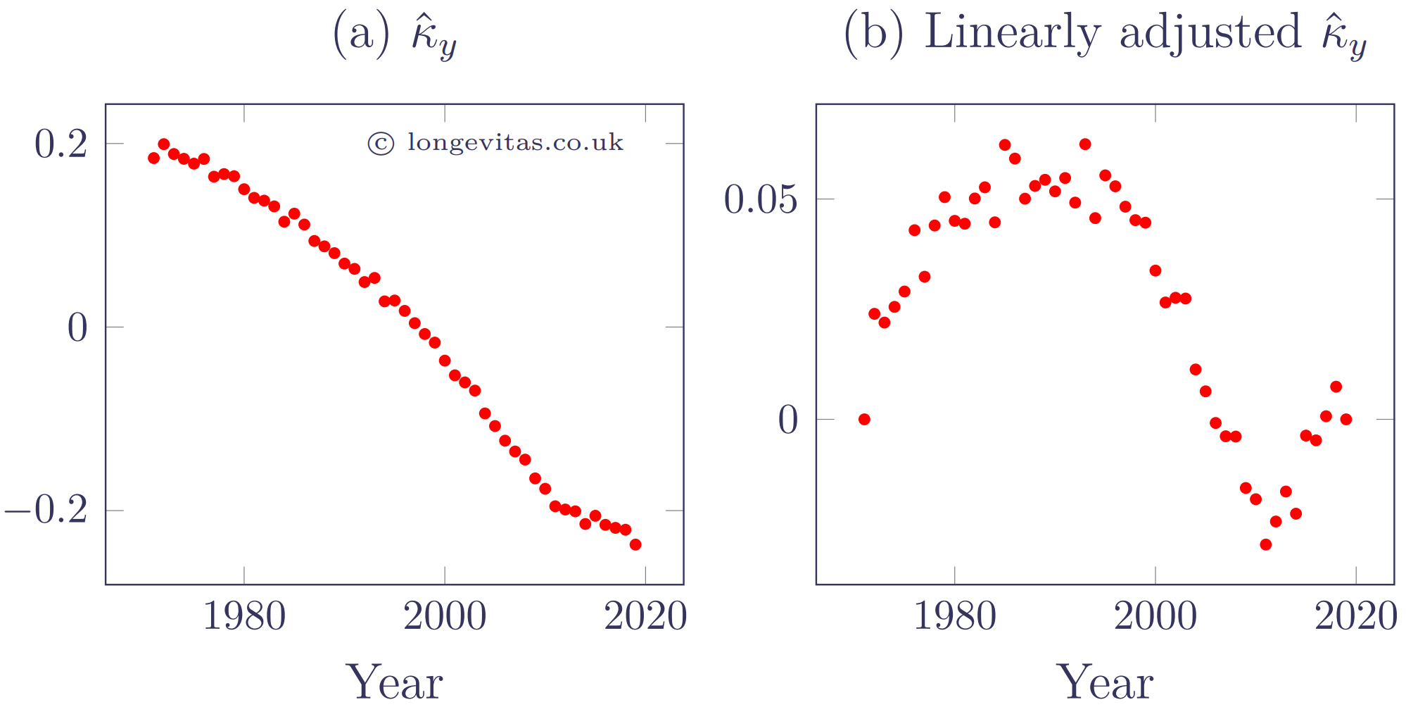
with appropriate identifiability constraints.  Figure 1 shows the estimated \(\hat\kappa_y\) in the left panel, which follow a vaguely linear pattern.  However, the linearly adjusted values of \(\hat\kappa_y\) are plotted in the right panel of Figure 1, showing that \(\hat\kappa_y\) goes on long meandering deviations around a possibly linear trend.

Figure 1.  \(\hat\kappa_y\) from Lee-Carter model fitted to mortality data for males in England & Wales, aged 50-105.  Source: own calculation using HMD data for 1971-2019.

It is clear from Figure 1(b) that \(\hat\kappa_y\) does not follow a strictly linear trend.  As a result, a common forecasting method, and the one used by Lee & Carter (1992), is a random walk with constant drift term \(\mu\):

\[\kappa_{y+1}=\kappa_y+\mu+\epsilon_{y+1}\qquad(2)\]

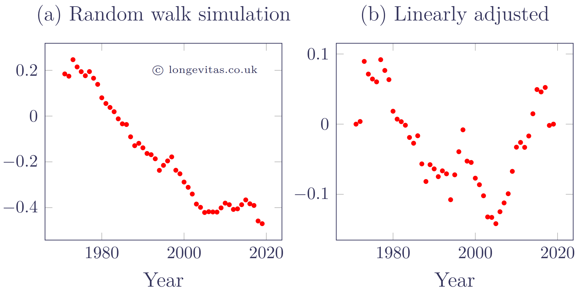
where \(\{\epsilon\}\) is a process of independent, identically distributed error term with zero mean and constant variance, \(\sigma^2\).  Starting with \(\hat\kappa_{1971}\) we can simulate a series using the \(\hat\mu=-0.00877\) and \(\hat\sigma^2=0.00107\) estimated from the \(\kappa_y\) values in Figure 1.  A single realisation of this random walk is shown on the left of Figure 2, along with the linearly adjusted  values on the right.

Figure 2.  Simulated \(\kappa_{y+t}\) values from \(y=1971\) onward (left panel) with linearly adjusted equivalents (right panel).  Source: own calculations.

The random walk with drift in Figure 2(a) has a rougher look to it than the \(\hat\kappa_y\) values in Figure 1(a), and it has produced faster overall improvements in this particular scenario.  Figure 2(b) exhibits similar long, meandering departures around the straight-line assumption, but with greater variability than in Figure 1(b).  We can see that equation (2) still has a straight line at its core by repeatedly applying the relationship for \(t\) years:

\[\kappa_{y+t}=\kappa_y+\mu t+\sum_{i=1}^t \epsilon_{y+i}\qquad(3)\]

which shows that under the random walk with drift, \(\kappa_{y+t}\) is a straight line (the \(\kappa_y+\mu t\) part) with a cumulative random walk overlay (the \(\sum_{i=1}^t\epsilon_{y+i}\) part).  We note that equation (2) can also be expressed as follows:

\[(1-B)\kappa_{y+t}=\mu+\epsilon_{y+t}\qquad(4)\]

where \(B\) is the backshift operator such that \(B\kappa_{y+t}=\kappa_{y+t-1}\).  If we define a linear process, \(\mu_t = t\mu\), then we can write equation (4) as:

\[(1-B)(\kappa_{y+t}-\mu_t)=\epsilon_{y+t}\qquad(5)\]

A comparison of Figures 1 & 2 suggests that we could improve on the simple random walk.  We now consider an ARIMA (\(p\), \(d\), \(q\)) model for \(\kappa_y\):

\[\phi(B)(1-B)^d(\kappa_{y+t}-\mu_t)=\theta(B)\epsilon_{y+t}\qquad(6)\]

where \(d\) is the level of differencing and \(\phi(B)\) and \(\theta(B)\) are polynomials in \(B\) of order \(p\) and \(q\), respectively.  Equation (6) is a generalisation of the random walk specified in equation (5).  However, the most common application in mortality work is with \(d=1\), in which case equation (6) can be re-arranged as follows:

\[\kappa_{y+t}=\kappa_y+t\mu+\frac{\theta(B)}{\phi(B)}\sum_{i=1}^t \epsilon_{y+i}\qquad(7)\]

As with the random walk, an ARIMA(\(p\), 1, \(q\)) model for \(\kappa_y\) is therefore composed of a straight line (the \(\kappa_y+t\mu\) part) and a moving-average overlay (the \(\phi^{-1}(B)\theta(B)\sum_{i=1}^t \epsilon_{y+i}\) part).  Equation (7) specifies a regression ARIMA model: the model is a straight-line linear regression with an ARIMA process for the deviations.

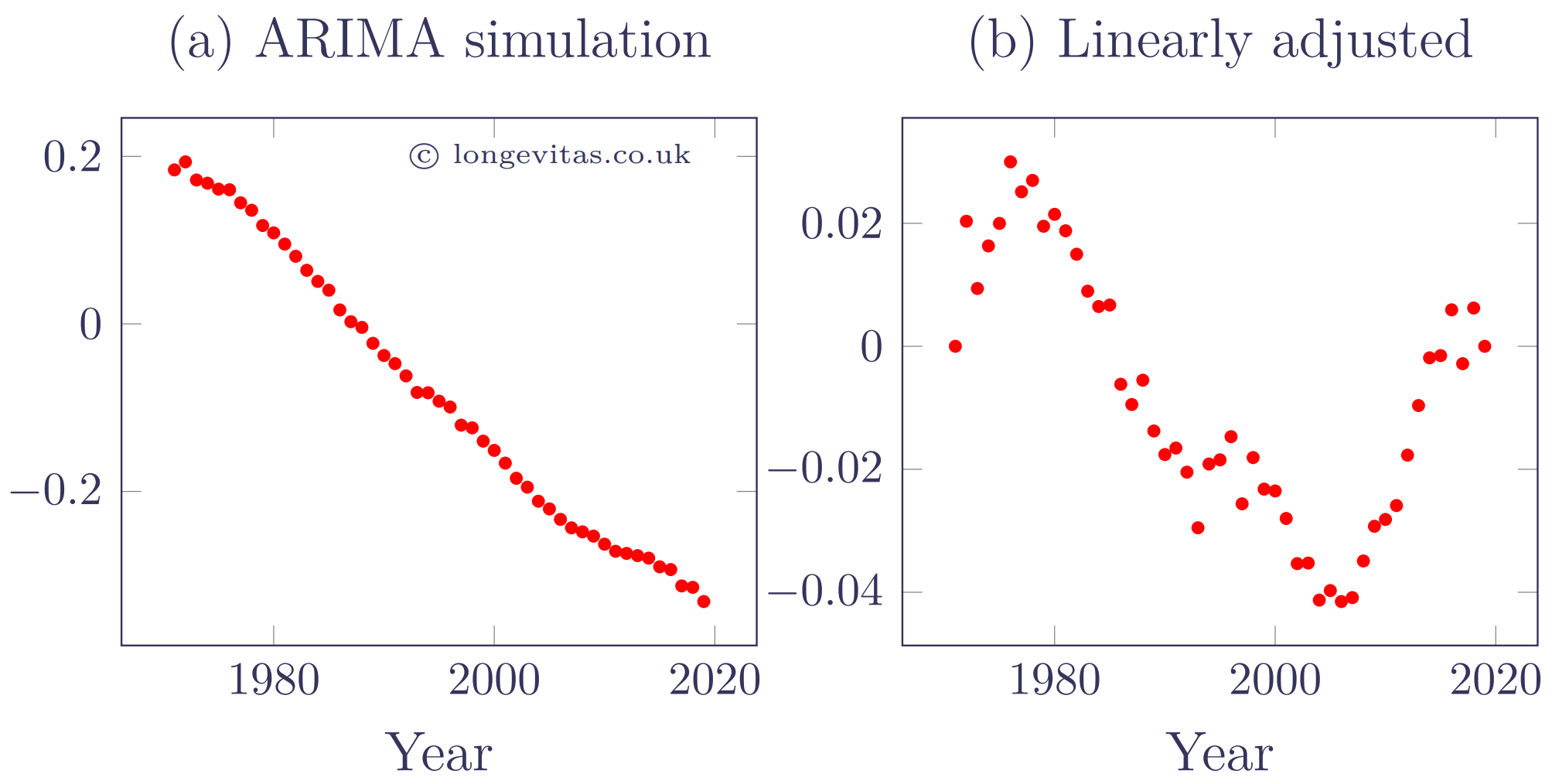
An ARIMA(1, 1, 2) model for \(\kappa_y\) is simulated in Figure 3 with \(\hat\phi_1=0.759247\), \(\hat\theta_1=-1.17789\) and \(\hat\theta_2=0.620675\).  The value for \(\hat\mu\) is the same as the random walk, as we are using the approach of Kleinow & Richards (2016).  However,  \(\hat\sigma^2\) is much smaller at \(0.00005461\).  For comparability the simulated \(\epsilon_{y+i}\) values are the same as used in Figure 2.

Figure 3.  ARIMA(1, 1, 2) simulation of \(\kappa_{y+t}\) values from \(y=1971\) onward (left panel) with linearly adjusted equivalents (right panel).  Source: own calculations.

Figure 3 shows that the ARIMA model does a better job of reproducing the look and feel of the actual \(\hat\kappa_{y+t}\) values in Figure 1.  Not only are the long meandering deviations from the linear reproduced, but there is a suitably higher degree of autocorrelation than exhibited by the random walk in Figure 2.  Of course, the better fit of an ARIMA model can best be quantified objectively using an information criterion.  However, the right-hand panels of Figures 1-3 provide a useful qualitative comparison.

Mortality trends are never quite linear, so linear models are neither the best fit nor the best means of forecasting.  However, random walks and ARIMA(\(p\), 1, \(q\)) models both have a linear foundation with an overlay that can reproduce the sort of correlated deviations in past mortality patterns.

References:

Kleinow, T. and Richards, S. J. (2016) Parameter risk in time-series mortality forecasts, Scandinavian Actuarial Journal, 2017, Issue 9, pages 804-828, doi 10.1080/03461238.2016.1255655.
Lee, R. D. and Carter, L. (1992) Modelling and forecasting the time series of U.S. mortality, Journal of the American Statistical Association, 87, pages 659-671.
Time-series models in the Projections Toolkit
Univariate forecasting models in the Projections Toolkit support both random walks (referred to as drift models) and ARIMA models for fitting, forecasting and generating sample paths.
The drift term, \(\mu\), is called the mean, and can be estimated one of two ways: integral with the other parameters (the Currie approach) or before the other parameters (the Kleinow-Richards approach). This can be controlled with the ARIMA Parameter Risk Method configuration option.
Add new comment