Up close and intimate with the APCI model
This blog brings together two pieces of work. The first is the paper we presented to the Institute and Faculty of Actuaries, "A stochastic implementation of the APCI model for mortality projections", which will appear in the British Actuarial Journal. The second is a previous blog where I examined the role of constraints in models of mortality. The present blog combines the two and looks at the application of constraints to the CMI's APCI model. I showed the results to a fellow statistician who expressed astonishment and even used the word "unbelievable"'. So buckle up, and prepare to be astonished!
We use data on UK males from the UK's Office for National Statistics. We have the number of deaths, \(d_{x,y}\), age \(x\) last birthday in year \(y\) and mid-year population estimates, the central exposures \(E^c_{x+1/2, y+1/2}\) for ages 50–100 and for years 1971–2015. We assume that \(D_{x,y}\), the random variable corresponding to the observed deaths \(d_{x,y}\), follows the Poisson distribution with mean \(E^c_{x+1/2, y+1/2}\mu_{x+1/2, y+1/2}\), where \(\mu_{x+1/2, y+1/2}\) is the force of mortality at exact age \(x+1/2\) and exact time \(y+1/2\).
The CMI's APCI model is:
\[\log\,\mu_{i+1/2,\,j+1/2} = \alpha_i + \kappa_j + \gamma_{c(i,j)} + \beta_i(\bar y - y_j)\qquad (1).\]
Here we index the ages \(i = 1,\ldots,n_a\), and the years \(j = 1,\ldots, n_y\), where \(n_a = 51\) is the number of ages and \(n_y = 45\) is the number of years. The cohorts are indexed from one to \(n_c = n_a+n_y-1 = 95\) with the oldest cohort in the first year assigned the index one. With this convention \(c(i,j)= n_a-i+j\).
The APCI model is clever, since it combines a linearized version of the Lee-Carter term \(\beta_i \kappa_j \approx \kappa_j + \beta_i(\bar y - y_j)\), with a cohort term \(\gamma_{c(i,j)}\). The model in this form is an example of a generalized linear model. The CMI then goes one step further and smooths \(\boldsymbol{\alpha}\), \(\boldsymbol{\kappa}\), \(\boldsymbol{\gamma}\) and \(\boldsymbol{\beta}\). Here the CMI and I part company. At the risk of teaching grandma to suck eggs, insurance is about the proper assessment of risk; smoothing the \(\boldsymbol{\kappa}\) and \(\boldsymbol{\gamma}\) terms suppresses the stochastic element of the model. Any resulting forecast of mortality will appear more certain than the data justify. Our paper puts the stochastic element back where it belongs. Smoothing \(\boldsymbol{\alpha}\) and \(\boldsymbol{\beta}\) does not affect the stochastic element in (1), but has the desirable property of producing more regular forecasts. We will smooth the \(\boldsymbol{\alpha}\) and \(\boldsymbol{\beta}\) terms. We use the method of \(P\)-splines (Eilers and Marx, 1996) with cubic \(B\)-splines and a second-order penalty on both \(\boldsymbol{\alpha}\) and \(\boldsymbol{\beta}\).
Here is the first surprise. Model (1) requires five constraints to enable unique estimates of the parameters to be found, but we only require four when \(\boldsymbol{\alpha}\) and \(\boldsymbol{\beta}\) are smoothed with a second-order penalty. There is an interaction between the model matrix and the penalty that reduces the effective rank of the model. This was completely unexpected. Note that this is a different point on identifiability constraints from the one made in Richards et al (2019) — there we observed that you do not need all five constraints if you don't estimate effects for corner cohorts. In fact both points are related mathematically, and a full explanation behind this behaviour is given in Currie (submitted).
The following four constraints achieve identifiability in the smooth version of (1):
\[\sum \kappa_j = \sum \gamma_c = \sum c \gamma_c = \sum c^2 \gamma_c = 0\qquad (2).\]
We refer to these constraints as the standard constraints.
However, the perverse soul from my previous blog is up to his old tricks and instead places four sets of random constraints on all the parameters. He argues that the choice of constraints doesn't make any difference to the estimates and forecasts of mortality, so a random set does the job just as well as a particular set such as (2). Estimates of the parameters under the standard constraints are denoted by suffix \(s\) as in \(\boldsymbol{\hat\alpha_s}\), and by suffix \(r\) as in \(\boldsymbol{\hat\alpha_r}\), for the random constraints.
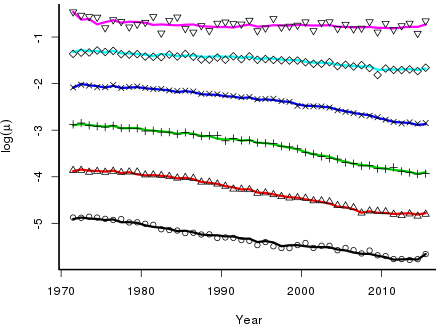
So what happens? Figure 1 shows the two sets of estimates. The estimates are spectacularly different in both shape and scale. Surely there is something wrong? Interestingly, no — Figure 2 shows the observed and fitted \(\log(\mu)\). Despite the differences in the estimated parameters, the fitted values under both sets of constraints are identical.
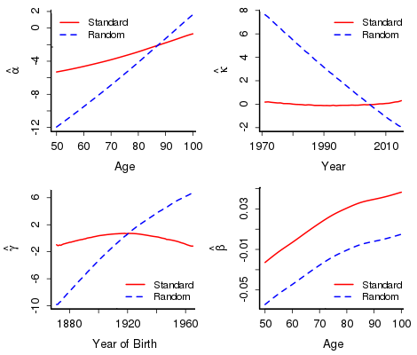
But there is more. Forecasting with an ARIMA model with either set of parameters gives identical forecasts. This seems a bit of a stretch, given the differences between the two sets of estimates. The point is that these estimates are closely related and these relationships orchestrate the behaviour of the forecasts. To be precise, the difference between \(\boldsymbol{\hat\beta_s}\) and \(\boldsymbol{\hat\beta_r}\) is a constant (here 0.0415) while the differences in the other sets are all linear; for example, here \(\boldsymbol{\hat\alpha_s} - \boldsymbol{\hat\alpha_r}=-0.1790 \times {\rm age} + 6.822\).
In conclusion, the two sets of estimates do much more than merely hold hands — they are up close and intimate, and this intimacy ensures that estimates and forecasts are inevitably identical. There is some very beautiful mathematics controlling this behaviour. There has been some discussion in the literature about the choice of constraints; for example, whether constraints on cohort parameters should be weighted by the number of times a cohort appears in the data. This discussion is now seen to be redundant. You can even follow the perverse soul and use random constraints!
References:
Currie, I. D. (in preparation). Constraints, the identifiability problem and the forecasting of mortality.
Eilers, P. H. C. and Marx, B. D. (1996). Flexible smoothing with B-splines and penalties, Statistical Science, 11, 89–121.
R Core Team (2018). R: A Language and Environment for Statistical Computing. R Foundation for Statistical Computing, Vienna, Austria. URL https://www.r-project.org/.
Richards, S. J., Currie, I. D., Kleinow, T. and Ritchie, G. P. (2019). A stochastic implementation of the APCI model for mortality projections, British Actuarial Journal (to appear).
Comments
Hi Iain
Thank you for posting your findings on APCI model.
I used different constraints available in Longevitas to check the sensitivity of these constraints to 1-year VaR capital requirement under SII when APCI model is used. I agree with you that despite the differences in the estimated parameters when different constraint schemes are used (as per to your figure 1), the fitted values are identical (as per to your figure 2). This is a good property in the case of CMI model as we use only the fitted values to determine the initial rates of improvements.
However, my analysis, based on Longevitas output, suggests that different constraints produce different forecasts resulting different best estimate and different capital requirements. I’m interested to know whether your independent analysis suggest the same. My analysis suggests, when APCI smoothed alpha and beta model is fitted to E&W combined males and female data then it could produce a difference in best estimate cohort expectation of Life of 0.5 years, when different constraint systems are used.
Kind regards
Kaushallya
Thank you Kaushallya for reading my blog on invariance and for your comments. In my blog, the models are fitted with the full set of age, period and, critically, cohort parameters. However, in the Toolkit we follow Cairns, Blake, Dowd et al (2009) and drop the effects for the corner cohorts. A consequence of this is that with the usual set of five constraints in the APCI model (or indeed any set of five independent constraints) the model is over-constrained. In practice this has worked well and models give very sensible forecasts. However, the beautiful invariance results which I describe will no longer hold.
One further thought. The treatment of corner cohorts, while very plausible based as it is on the number of cells contributing to a particular cohort, pays closer examination. For example, in my data-set, the youngest cohort (age 50 in 2015), has 1621 deaths with an exposure of 465548. This gives a point estimate of the force of mortality of 1621/465548 = 0.00348 and standard error the square root of 0.00348/465548 = 0.00009. In contrast, the oldest cohort (age 100 in 1970) has 58 deaths and an exposure of 92. The corresponding values are 0.630 with standard error 0.083. Thus the youngest cohort (whose effect we certainly wish to forecast) is well estimated while the oldest cohort (whose effect does not enter into any forecast) is poorly estimated. This argument can be made very much more precise (see Corollary 2 in the Appendix to my 2013 paper ). I will return to this topic later in the year.
References
Cairns, Blake, Dowd et al (2009) North American Actuarial Journal, vol 13, p1-35.
Currie (2013) Statistical Modelling, vol13, p69-93.
Add new comment