Signal or noise?

Each year since 2009 the CMI in the UK has released a spreadsheet tool for actuaries to use for mortality projections. I have written about this tool a number of times, including how one might go about setting the long-term rate. The CMI now wants to change how the spreadsheet is calibrated and has proposed the following model in CMI (2016a):

\[\log m_{x,y} = \alpha_x + \beta_x(y-\bar y) + \kappa_y + \gamma_{y-x}\qquad (1)\]

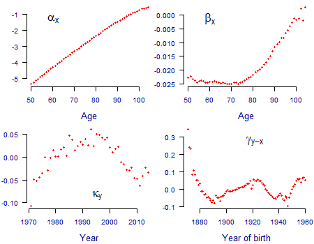
which the CMI calls the APCI model. \(m_x\) is the central rate of mortality at age \(x\) in year \(y\) and \(\alpha_x\), \(\beta_x\), \(\kappa_y\) and \(\gamma_{y-x}\) are vectors of parameters to be estimated. \(\bar y\) is the average year, which is used to centre the time index around zero. The APCI model needs five constraints for the parameters to be identifiable. The estimated parameters for males in England & Wales over 50 are shown in Figure 1; all data were used but cohort terms were not estimated for years of birth with fewer than five observations. Unlike the CMI we have not applied smoothing to the parameters, for reasons we will come to at the end of this article.

Figure 1. Parameter estimates for APCI model. Source: own calculations using unsmoothed model fitted to ONS population data for males in England & Wales for 1971-2014 for ages 50-104.

The APCI model has some apparent similarities to other models, including the Age-Period (AP), Age-Period-Cohort (APC) and Lee-Carter (LC) models:

\[\begin{align} {\rm AP}\quad \log m_{x,y} &= \alpha_x + \kappa_y \\ {\rm APC}\quad \log m_{x,y} &= \alpha_x + \kappa_y + \gamma_{y-x} \\ {\rm LC}\quad \log m_{x,y} &= \alpha_x + \beta_x\kappa_y\end{align}\]

As with the APCI model, these models also need constraints for the parameters to be identifiable: the AP model needs one, the Lee-Carter model needs two and the APC model needs three. In all four models some parameters perform equivalent functions: for example \(\alpha_x\) is broadly the average value of \(\log m_{x,y}\) over time, while \(\gamma_{y-x}\) is a cohort term which is intended to follow year-of-birth patterns. However, \(\kappa_y\) in the APCI model performs a different role to the equivalently named parameter in the other three models, as illustrated in Figure 2.

Figure 2. Estimated values of \(\kappa\) for Age-Period, APC and Lee-Carter models. Source: own calculations using unsmoothed models fitted to ONS population data for males in England & Wales for 1971-2014 for ages 50-104.

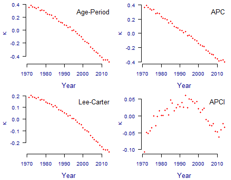
The Age-Period, APC and Lee-Carter models are designed for forecasting, and the principle way of doing this is to forecast \(\kappa_y\). In all three cases there is a relatively clear, consistent trend in Figure 2 that can be forecast, either using a drift model or (better) an ARIMA model.

In contrast \(\kappa_y\) in the APCI model is not the whole story for forecasting, at least not directly and not in the same way as the others. The comparison of \(\kappa\) for the APCI model with the others in Figure 2 shows one reason why: there is much less of an obvious trend or signal in \(\kappa\) to forecast. This is because the \(\beta_x(y-\bar y)\) term in the APCI model in equation (1) has extracted much of the trend exhibited by \(\kappa\) in the other three models, leaving \(\kappa\) in the APCI model to pick up any residual curvature and random error. As a result, \(\kappa\) under the APCI has a less-clear structure to forecast than for the other models.

The difference is important because the CMI (2016a, 2016b) proposes to use smoothed values of \(\kappa\) in setting the initial rates of mortality improvement in its next generation of its spreadsheet tool (known as CMI_2016 and scheduled for final release in March 2017). Unlike in Figure 1, the CMI fits the APCI model in equation (1) with smoothing on each of the four parameter sets. In particular, the CMI smooths \(\kappa\) with a hyperparameter, \(S_\kappa\), and the CMI made the following observation in CMI (2016b):

"life expectancies are [...] very sensitive to the choice made for \(S_\kappa\), with the impact varying across the age range. At ages above 45, changing \(S_\kappa\) by 1 has a greater impact than changing the long-term rate by 0.5%."

CMI (2016b), page 42.

The APCI panel in Figure 2 shows why \(S_\kappa\) is so influential: there is a lot more relative noise in \(\kappa\) under the APCI model, and the pattern from 2010 onwards is not an obvious continuation of the pattern in the two decades prior to 2010. As a result, lighter or heavier degrees of smoothing will lead to potentially large changes in the direction taken by \(\kappa\) for years after 2010. Since the smoothed values of \(\kappa\) are used to help set the starting rates of mortality improvement in the CMI spreadsheet, the value of \(S_\kappa\) has a large impact on the projection scenario.

References:

CMI (2016a) CMI Mortality Projections Model consultation, Working Paper 90.
CMI (2016b) CMI Mortality Projections Model consultation — technical paper, Working Paper 91.
Add new comment