Parameterising the CMI projection spreadsheet
The CMI is the part of the UK actuarial profession which collates mortality data from UK life offices and pension consultants. Amongst its many outputs is an Excel spreadsheet used for setting deterministic mortality forecasts. This spreadsheet is in widespread use throughout the UK at the time of writing, not least for the published reserves for most insurers and pension schemes.
Following Willets (1999), the basic unit of the CMI spreadsheet is the mortality-improvement rate:
\[1 - \frac{q_{x,t}}{q_{x,t-1}}\qquad(1)\]
where \(q_{x,t}\) is the probability of death aged \(x\) in year \(t\), assuming a life is alive at the start of the year.
The CMI spreadsheet contains over a thousand user-variable parameters that are supplied with default values derived from population data. There is a lot which could be improved here, such as using smoothing to reduce the effective number of parameters. However, there is one parameter which the CMI purposefully does not pre-populate: the assumed long-term rate of improvement (LTR). The CMI provides no guidance as to what value to use here, which forces users to make their own assessment.
So how can a user set the LTR? This is a forward-looking parameter that is not directly calibrated to data, so looking to past mortality experience may be of limited relevance. Equally, the setting of the LTR is as much about expert judgement as anything else, so a formal model- or data-driven approach is not the only way of approaching such a subjective decision. However, without data or statistical model, one needs to be very careful when picking a value for such a parameter. Even experts in the field can get these sorts of assumptions wrong.
Nevertheless, many users would prefer some kind of quantitative approach, not least when actuaries have to justify their assumptions to auditors and regulators. One simple approach would be to start with the best-known mortality model of them all, i.e. the Lee-Carter model:
\[ \log \mu_{x,t} = \alpha_x + \beta_x\kappa_t\qquad(2)\]
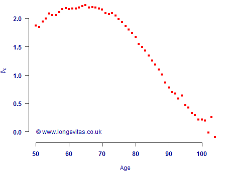
where the parameters \(\alpha_x\), \(\beta_x\) and \(\kappa_t\) are to be estimated. This model can be fitted easily enough, subject to the specification of two constraints and some awareness of the behaviour of the parameters in a constrained model. Figure 1 shows the estimated age-related response, \(\hat\beta_x\), to the estimated period effect, \(\hat\kappa_t\) (not shown). The \(\hat\beta_x\) values are for males in England & Wales spanning a period of 43 years.
We can take equation (2) and use it to express the mortality-improvement rate in equation (1) in terms of the Lee-Carter parameters:
\[\begin{align}
1-\frac{q_{x,t}}{q_{x,t-1}} &\approx 1 - \frac{\mu_{x,t}}{\mu_{x,t-1}} \\
&= 1 - \frac{e^{\alpha_x+\beta_x\kappa_t}}{e^{\alpha_x+\beta_x\kappa_{t-1}}} \\
&= 1 - e^{\beta_x(\kappa_t-\kappa_{t-1})}\qquad(3)\end{align}\]
By expanding equation (3) as a Maclaurin series, we get the following approximation:
\[1-\frac{q_{x,t}}{q_{x,t-1}} \approx -\beta_x (\kappa_t-\kappa_{t-1})\qquad(4)\]
We now have an approximation for the mortality-improvement rate which just involves \(\beta_x\) and \(\kappa_t\). The next step is to specify a model for projection, of which the simplest is a random walk with drift, i.e.
\[\kappa_{t} - \kappa_{t-1} = m + \epsilon_t\qquad(5)\]
where \(m\) is the drift constant and \(\epsilon_t\) is a random error term with zero mean. Taking expectations and substituting equation (5) into equation (4) gives an approximation for the mortality-improvement rate using only \(\hat\beta_x\) and \(\hat m\):
\[1-\frac{q_{x,t}}{q_{x,t-1}} \approx -\hat\beta_x\hat m\qquad(6)\]
Using the same data set as in Figure 1, Kleinow & Richards (2016) estimated \(\hat m = -0.011176\). Using equation (6) and the \(\hat\beta_x\) values in Figure 1 we can then calculate the mortality-improvement rates implied by the model, as in Figure 2. The shape is obviously the same as in Figure 1 — we have just multiplied \(\hat\beta_x\) by a constant, \(\hat m\) — and we have expressed the resulting mortality-improvement rates as percentages.
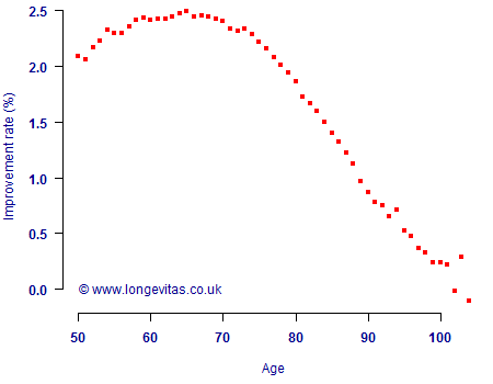
We are finally at a point where we can think about the LTR for the CMI spreadsheet. What value should we use? The improvement rates in Figure 2 lie between 2% and 2.5% p.a. from ages 50 to 78 inclusive, but fall sharply towards zero above age 100. Since annuity liabilities are typically concentrated in the 65-80 age range, an insurer might start with an LTR of 2% and adjust for circumstances. However, it is an open question as to whether it makes sense to take parameters from one model — \(\hat\beta_x\) and \(\hat m\) in this case — and use them to inform a parameter value in a quite different model.
References:
Kleinow, T. and Richards, S. J. (2016) Parameter risk in time-series mortality forecasts, Longevitas Ltd.
Willets, R. C. (1999) Mortality in the next millennium, Staple Inn Actuarial Society, London.
Add new comment