Constraints and the R language
This is the fourth and final blog on the use of constraints in the modelling and forecasting of mortality. The previous three blogs (here, here and here) demonstrated that there is no need to worry about which linear constraints to use: the fitted values of mortality and crucially their forecast values always come out the same. In this blog I thought it would be both interesting and instructive to see how the R language deals with models with non-identifiable parameters.
We will illustrate the ideas with the age-period-cohort or APC model fitted to male data from the Office for National Statistics. We have the number of deaths, \(d_{x,y}\), age \(x\) last birthday in year \(y\) and corresponding mid-year population estimates, the central exposures \(E^c_{x+1/2, y+1/2}\), for ages 50–104 and years 1971–2015. For convenience we use age indices \(1,\ldots,n_a\) and year indices \(1,\ldots,n_y\). We assume the oldest cohort in the first year is indexed 1 and so the cohort index at age \(x\) in year \(y\) is \(c(x,y) = n_a - x + y\). For our data we have \(n_a = 55\) ages, \(n_y = 45\) years and \(n_c = 99\) cohorts. We assume that the number of deaths follows a Poisson distribution with mean \(E^c_{x+1/2, y+1/2}\, \mu_{x+1/2, y+1/2}\) where \(\mu_{x+1/2,y+1/2}\) is the force of mortality at exact age \(x+1/2\) and exact year \(y+1/2\). The APC model is
\[\log \mu_{x+1/2,y+1/2} = \alpha_x + \kappa_y + \gamma_{c(x,y)},\,x =1,\ldots,n_a,\,y = 1,\ldots,n_y\quad(1).\]
The APC model is an example of a very wide class of models, a generalized linear model or GLM (McCullagh and Nelder, 1989). The glm() command in the R language fits a GLM. We specify the model matrix, \(\boldsymbol{X}\). For the APC model we have
\[\boldsymbol{X} = [\boldsymbol{X_a} : \boldsymbol{X_y} : \boldsymbol{X_c}], \; n_an_y \times (n_a+n_y+n_c)\qquad\qquad(2).\]
There are \(n_an_y\) observations and \(n_a+n_y+n_c\) parameters. Each row of \(\boldsymbol{X}\) consists of three ones which pick out the corresponding age, year and cohort parameters; the remaining entries are zero. For example, the first row of \(\boldsymbol{X}\) corresponds to the youngest age, \(i = 1\), the first year, \(j=1\) and the cohort \(n_a -1+1 = n_a\), and has a one in the first position, a one in the \(n_a+1\) position and a one in the \(2n_a+n_y\) position. Currie (2016) gives examples of model matrices for some common models of mortality and the code on the right gives the construction of \(\boldsymbol{X}\) for the APC model.
We suppose that the R objects Dth and Exp contain the vectors of observed deaths and exposures, and that X contains the model matrix. With this setup we fit the APC model with the single line of R
Fit.GLM <- glm(Dth ~ X + offset(log(Exp)), family=poisson) (3)
where the exposures enter into the code as an offset; see Macdonald et al (2018, section 10.8) for a careful discussion of offsets. The R object Fit.GLM contains a wealth of information on our fitted model; names(Fit.GLM) lets you see what is available. The fitted regression coefficients are in Fit.GLM$coef and here we get our first surprise: by default, R has fitted an intercept term. We have fitted the APC model in the form
\[\log \mu_{x+1/2,y+1/2} = \theta_0 + \alpha_x + \kappa_y +\gamma_{c(x,y)},\,x = 1,\ldots,n_a,\,y = 1,\ldots,n_y\quad(4),\]
where \(\theta_0\) is the intercept. We can suppress the intercept with
Fit.GLM <- glm(Dth ~ -1 + X + offset(log(Exp)), family=poisson)} (5)
We know that the parameters in the APC model are not identifiable; three constraints are needed to give unique estimates. How does R treat this problem? Inspection of the fitted coefficients in Fit.GLM$coef computed with (5) reveals that parameters 100, 198 and 199 are reported as NA, ie, not available; these parameters correspond to the final period parameter, \(\kappa_{45}\) and the final two cohort parameters \(\gamma_{98}\) and \(\gamma_{99}\). R has been ruthless in its treatment of the identifiability problem: if the parameters are not identifiable then it simply does not estimate some subset of them.
What has R done? The glm() call was provided with the model matrix, \(\boldsymbol{X}\). R scans the columns of \(\boldsymbol{X}\) from left to right and checks if the current column is linearly dependent on the previous columns. All is well until we reach the column corresponding to the final period parameter; this column is linearly dependent on the previous columns. R deletes this column from \(\boldsymbol{X}\) and takes a note of the deletion. R now repeats this procedure and deletes the columns corresponding to the final two cohort parameters. We end up with (a) a model matrix of full rank whose remaining coefficients are uniquely estimable and (b) a list of deleted columns. The model is fitted, the estimated coefficients are reported and the deleted coefficients are slotted in as NA.
I very much like this approach. There is something refreshingly honest about it! If something is not estimable R does not attempt by some arbitrary assumption (such as the use of constraints) to estimate it.
What is the connection between the approach to identifiability used by R and that often used by actuaries? We can mimic R's method with the constraints
\[\kappa_y = \gamma_{n_c-1} = \gamma_{n_c} = 0\qquad\qquad(6),\]
ie, we constrain the final period parameter and the final two cohort parameters to be zero. It is hard to see an argument to support this choice, unlike the standard choices of constraints made, for example, in Cairns et al (2009). We refer to these constraints, implicit in R's approach, as the R constraints. We fit the model with the constraints (6). The fitted coefficients are precisely those in Fit.GLM$coef but with the NA values replaced by zeros.
Invariance is a powerful and fundamental idea. One consequence is that we can compute any constrained fit from any given fit. For example, the R code in (3) and (5) both give the invariant fitted values of \(\log \hat \mu_{i,j}\). Currie (to appear) gives the following formula for the estimated regression coefficients subject to a particular set of constraints
\[\hat {\boldsymbol{\theta}} = (\boldsymbol{X}^\prime \boldsymbol{X} + \boldsymbol{H}^\prime \boldsymbol{H})^{-1} \boldsymbol{X}^\prime \log \hat {\boldsymbol{\mu}}\qquad\qquad(7)\]
where \(\boldsymbol{\theta}\) is the vector containing the stacked coefficients \(\boldsymbol{\alpha}\), \(\boldsymbol{\kappa}\) and \(\boldsymbol{\gamma}\), \(\boldsymbol{H}\) is the constraints matrix that defines the given constraints and \(\hat {\boldsymbol{\mu}}\) is the vector of invariant forces of mortality computed from (3) or (5). The vector \(\hat {\boldsymbol{\theta}}\) now contains the estimated regression coefficients subject to the constraints defined by \(\boldsymbol{H}\). We note that we do not need to know what (implicit) constraints R has used to compute \(\log \hat {\boldsymbol{\mu}}\).
For example, in the APC model Cairns et al (2009) use the constraints
\[\sum_{j=1}^{n_y} \kappa_j = \sum_{c=1}^{n_c} \gamma_c =\sum_{c=1}^{n_c} c \gamma_c = 0\qquad(8)\]
which we refer to as the standard constraints. In this case, the constraints matrix \(\boldsymbol{H}\) is \(3 \times (n_a+n_y+n_c)\); the R code on the right also gives the construction of \(\boldsymbol{H}\) for the APC model.
The usual approach is to apply the constraints as part of the estimation algorithm for \(\boldsymbol{\theta}\). Invariance allows us to ignore the constraints completely and use the glm() function to compute the invariant fit. If required, any constraints can be applied as an afterthought.
Figure 1. Estimated regression coefficients subject to the standard constraints (8) and R's constraints (6). Observed and invariant fitted \(\log \hat {\boldsymbol{\mu}}\) for age 65.
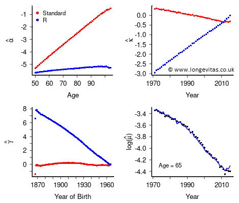
Figure 1 shows the estimated coefficients under the R constraints (6) and the standard constraints (8); they are strikingly different. The bottom right panel shows the invariant fitted values of \(\log \hat {\boldsymbol{\mu}}\) computed under the constraints (6) or (8), or indeed any set of linear constraints.
Invariance is a profound idea and can be used in ways that are perhaps unexpected. In this mini-series of blogs we have discussed the influence of invariance on (a) forecasting, (b) the APCI model and (c) standard errors. In this final blog, we have shown how invariance can be used to bypass the use of constraints during the estimation stage. Mathematicians can often be accused of being obsessed with an idea. I confess that over the last two years invariance has been something of an obsession with me, and I don't think I'm done yet. Watch this space!
References:
Cairns, A. J. G., Blake, D., Dowd, K., et al. (2009). A quantitative comparison of stochastic mortality models using data from England and Wales and the United States. North American Actuarial Journal, 13, 1–35.
Currie, I. D. (2016). On fitting generalized linear and non-linear models of mortality. Scandinavian Actuarial Journal, 2016, 356–383.
Currie, I. D. (to appear). Constraints, the identifiability problem and the forecasting of mortality. Annals of Actuarial Science.
Macdonald, A. S., Richards, S. J. and Currie, I. D. (2018). Modelling Mortality with Actuarial Applications. Cambridge: Cambridge University Press.
McCullagh, P. and Nelder, J. A. (1989). Generalized Linear Models, London: Chapman and Hall.
R Core Team (2019). R: A Language and Environment for Statistical Computing. R Foundation for Statistical Computing, Vienna, Austria. URL https://www.R-project.org/.
Previous posts
From magical thinking to statistical thinking
Matrix repair
When fitting a statistical model we want two things as a minimum:
Add new comment