M is for Estimation

In earlier blogs I discussed two techniques for handling outliers in mortality forecasting models:

• Chen & Liu (1993) for ARIMA models for univariate time series, and

• Galeano, Peña & Tsay (2006) for multivariate random walks.

There is a triple benefit to these procedures:

1. The identification of outliers is objective, based on statistical tests.

2. Having identified the outliers, their effect can be co-estimated with the model parameters to reduce bias.

3. If the most recent years are affected by outlier effects, robust starting points for the forecast can be calculated by simply deducting the outlier effects.

In the case of Chen & Liu (1993), there is a fourth benefit: the nature of the outlier can be classified.

However, during a recent presentation I was asked about  the older technique of likelihood robustification.  This has been superseded for time-series work, but it might be of historical interest to some readers; enthusiasts can consult the likes of Martin, Samarov & Vandaele (1982) for robustified likelihoods for ARIMA models.

To illustrate likelihood robustification in general, consider the contribution of a single data point, $x$, to the likelihood for a N(0,1) random variable:

\[L\propto \frac{1}{\sqrt{2\pi}}e^{-\frac{1}{2}x^2}\qquad(1)\]

Multiplicative factors involving only constants don't affect inference, so the contribution to the log-likelihood is therefore:

\[\ell = \log L = -\frac{1}{2}x^2\qquad(2)\]

In the literature on likelihood robustification it is the convention to minimise the negative log-likelihood, so we work with:

\[-\ell = \frac{1}{2}x^2\qquad(3)\]

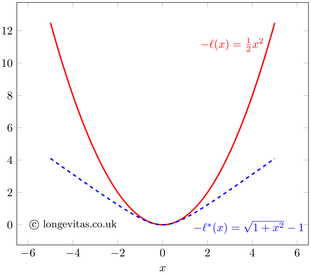
The function $-\ell$ is plotted as the solid line in Figure 1.  In this form it is referred to as a loss function.  The contribution to the log-likelihood increases quadratically with $x$.  We know that 95% of N(0,1) variates lie in (-1.96, 1.96), so an outlier value of 5 (say) will have a large and distorting influence on inference using the standard quadratic loss function.

Figure 1. Quadratic loss function, $-\ell$, and pseudo-Huber loss function, $-\ell^*$.

Huber (1964) introduced the idea of a loss function that behaved like equation (3) for non-outliers, but which restricted the contribution made by more extreme observations.  The term used for inference here is M-estimation, of which the maximum-likelihood estimate is a special case.  Specifically, to counter the distorting influence of outliers we replace the quadratic loss function in equation (3) with a function without an exponentially increasing influence.  There are many examples in the literature, but one is:

\[-\ell^* = \delta\left(\sqrt{1+(x/\delta)^2}-1\right)\qquad(4)\]

which is also plotted in Figure 1 for $\delta=1$.  The robustified function $-\ell^*$ behaves much like $-\ell$ in the region (-1, 1), but outliers outside (-2, 2) clearly have much less influence under $-\ell^*$ than under $-\ell$.  Thus, a robustified alternative to the log-likelihood can be constructed with an appropriate choice of loss function and any accompanying parameter (like $\delta$ in equation (4)).  Such methodologies still have their place in statistics, but the methodologies of Chen & Liu (1993) and Galeano, Peña and Tsay (2006) are preferred for time-series work for the reasons stated at the start.

References:

Chen, C. and Liu, L-M. (1993) Joint Estimation of Model Parameters and Outlier Effects in Time Series, Journal of the American Statistical Association, March 1993, Vol. 88, No. 421, pages 284–297.
Galeano, P., Peña, D. and Tsay, R. S. (2006) Outlier Detection in Multivariate Time Series by Projection Pursuit, Journal of the American Statistical Association, June 2006, Vol. 101, No. 474, pages 654–669.
Huber, P. (1964) Robust Estimation of a Location Parameter, The Annals of Mathematical Statistics, Vol. 35, No 1, March 1964, pages 73-101.
Martin, R. D., Samarov, A. and Vandaele, W. (1982) Robust methods for ARIMA models, Department of Statistics, University of Washington, Seattle, March 1982, Technical Report No. 21.
Add new comment