Compare and contrast: VaR v. CTE
Insurance reserving in many countries looks at extreme scenarios over a single year. The idea is that the insurer faces an uncertain liability, as represented by a random variable, \(X\) say. The question is then how to set a reserve for this liability, \(V_\alpha(X)\)? In this blog we consider two common regulatory approaches to setting \(V_\alpha(X)\):
- Value-at-risk (VaR). This is a quantile-based approach, i.e. \(V_\alpha(X)=Q_\alpha(X)\), where \(Q_\alpha(X)\) is the \(\alpha\)-quantile of \(X\), i.e. \(\Pr[X\leq Q_\alpha(X)]=\alpha\). The quantile approach to reserving underlies Solvency II in the European Union. The reserve \(V_\alpha(X)\) is thus set so that the liability \(X\) will be covered with a sufficiently high probability, \(\alpha\).
- Conditional Tail Expectation (CTE). This is the average value of \(X\), conditional on an extreme event having occurred, i.e. \(V_\alpha(X)=CTE_\alpha(X)\), where \(CTE_\alpha(X)={\rm E}[X|X>Q_\alpha(X)]\). The CTE approach to reserving underlies the Swiss Solvency Test (SST). Here the reserve \(V_\alpha(X)\) has a slightly different interpretation, namely that it should cover the average cost of an extreme event happening with probability \(\alpha\).
\(Q_\alpha(X)\) and \(CTE_\alpha(X)\) are obviously related, since \(CTE_\alpha(X)\geq Q_\alpha(X)\) for any distribution of \(X\). However, what if two territories each use the two different approaches with different values of \(\alpha\)? For example, under Solvency II insurers use VaR with \(\alpha=0.995\) (VaR99.5%), whereas under the SST insurers use CTE with \(\alpha=0.99\) (CTE99%). How comparable are the reserving levels for longevity trend risk when both the methodology and the value of \(\alpha\) differ?
To compare and contrast the two reserving approaches for longevity trend risk in immediate annuities, we will consider three alternative forecasting models: the model from Lee & Carter (1992), the Age-Period-Cohort model and the model from Cairns, Blake & Dowd (2006). These models are summarised below:
| Model | Expression |
|---|---|
| Lee-Carter, LC(S): | \(\log \mu_{x,y}=\alpha_x+\beta_x\kappa_y\) |
| Age-Period-Cohort, APC(S): | \(\log \mu_{x,y}=\alpha_x+\kappa_y+\gamma_{y-x}\) |
| Cairns-Blake-Dowd, M5(S): | \(\log \mu_{x,y}=\kappa_{0,y}+\kappa_{1,y}\)S(x) |
where \(\alpha_x\), \(\beta_x\), \(\kappa_y\), \(\kappa_{0,y}\), \(\kappa_{1,y}\) and \(\gamma_{y-x}\) are parameters to be estimated by the method of constrained maximum likelihood. \(S(x)\) is a P-spline-smoothed function of age, as are \(\alpha_x\) and \(\beta_x\); besides being intuitively reasonable, such smoothing also improves the forecasting performance for the Lee-Carter model. The labelling of the models with (S) serves as a reminder that these are all smoothed models. Identifiability constraints are required for all three models, but, as Iain showed in an earlier blog, these make no difference to the projections (which are done using ARIMA models for the Lee-Carter & APC models, and a bivariate random walk for M5).
We use the framework from Richards et al (2014) to generate the one-year distribution of annuity liabilities. Finally, we calculate the capital requirements for annuities in payment relative to the best-estimate, i.e. the relative capital requirement, \(C_\alpha(X)\), is given by:
\[C_\alpha(X) = \left[\frac{V_\alpha(X)}{{\rm E}[X]}-1\right]*100\%.\]
The results using UK population data are shown in Figures 1, 2 & 3, where the models are fitted separately for males and females.
Figure 1. Capital requirements for one-year longevity trend risk under LC(S) model. Source: Harrell-Davis estimate for \(Q_\alpha\) using 5,000 simulations of models fitted to UK data for ages 50–104, 1971–2016. Cashflows discounted at 2% per annum.
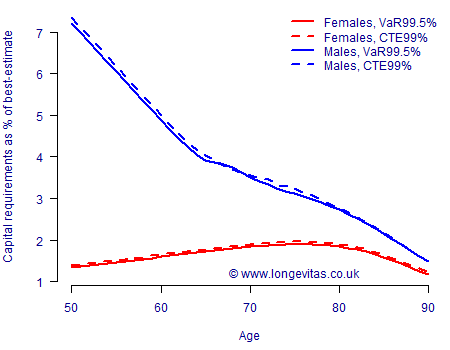
Figure 2. Capital requirements for one-year longevity trend risk under APC(S) model. Source: Harrell-Davis estimate for \(Q_\alpha\) using 5,000 simulations of models fitted to UK data for ages 50–104, 1971–2016. Cashflows discounted at 2% per annum.
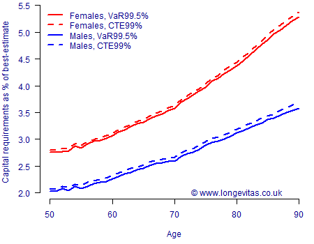
Figure 3. Capital requirements for one-year longevity trend risk under M5(S) model. Source: Harrell-Davis estimate of \(Q_\alpha\) using 5,000 simulations of models fitted to UK data for ages 50–104, 1971–2016. Cashflows discounted at 2% per annum.

A comparison of Figures 1, 2 & 3 tells us quite a bit:
- Model risk. Both the absolute level and the shape of capital requirements by age vary a lot among these three common models. Any assessment of capital requirements not only requires multiple unrelated models, it also demands allowance for the distribution of liabilities by age.
- Gender risk. This could be viewed as sub-variant of model risk: compared to female annuitants the capital requirement for male annuitants is either far higher (Lee-Carter model, Figure 1), far lower (Age-Period-Cohort model, Figure 2) or practically the same (CBD model, Figure 3). It is clear that one cannot just blindly apply the capital requirements for one gender to the other.
- Reserving approach. The CTE99% capital requirements are almost always higher than the VaR99.5% ones. That said, the reserve percentages are surprisingly close, with there typically being less than 0.1% difference between the two approaches.
Figures 1–3 show considerable variability, but there is one constant: VaR99.5% and CTE99% results for one-year longevity trend risk are closely comparable. This finding also applies to deferred annuities for UK lives, and also to Netherlands data for both immediate and deferred annuities (there is not the space here to show the corresponding graphs, but then can be found here). There are numerous other technical differences between the SST and Solvency II that make final published reserves much harder to compare; see Kinrade & Coatesworth (2013). However, the results here suggest that raw CTE99% and VaR99.5% outputs can at least be benchmarked against each other.
References:
Cairns, A. J. G. and Blake, D. and Dowd, K. (2006) A two-factor model for stochastic mortality with parameter uncertainty: theory and calibration, Journal of Risk and Insurance, 73, 687–718.
Kinrade, N. and Coatesworth, W. (2013) How equivalent are the quantitative aspects of Swiss Solvency Test and Solvency II for life insurers?, Milliman.
Lee, R. D. and Carter, L. (1992) Modeling and forecasting US mortality, Journal of the American Statistical Association, 87, 659–671.
Richards, S. J., Currie, I. D. and Ritchie, G. P. (2014) A value-at-risk framework for longevity trend risk, British Actuarial Journal, 19(1), 116–167 (with discussion).
Previous posts
Up close and intimate with the APCI model
This blog brings together two pieces of work. The first is the paper we presented to the Institute and Faculty of Actuaries, "A stochastic implementation of the APCI model for mortality projections", which will appear in the British Actuarial Journal. The second is a previous blog where I examined the role of constraints in models of mortality.
Add new comment