Modelling improvements in experience data - II
In my previous blog I looked at the implied mortality improvements from time-varying traditional actuarial survival models. In this blog we consider the implied improvements under the newer Hermite-spline model I proposed in Richards (2019). This paper included an explicit attempt to model age-related mortality changes, as discussed in this blog.
However, the Hermite-spline family also offers an alternative approach to time-varying mortality, one that is analogous to the approach under traditional actuarial models. We start by recapping the non-time-varying Hermite-spline model as follows for \(x\in [x_0, x_1]\) and \(t=(x-x_0)/(x_1-x_0)\):
\[\log\mu_x = \alpha h_{00}(t) + m_0 h_{10}(t) + \omega h_{01}(t) + m_1 h_{11}(t)\qquad(1)\]
where the \(h\) functions are the Hermite-spline functions shown here. \(\alpha\) is log(mortality) at age \(x_0\) and \(\omega\) is log(mortality) at age \(x_1\). Richards (2019) extended this to a time-varying model by explicitly adding an age-related improvement term. However, in a recent working paper (Richards, 2020) I extended equation (1) by replacing \(\alpha\) and \(m_0\) with time-varying functions as follows:
\[\log\mu_{x,y} = \alpha(y) h_{00}(t) + m_0(y) h_{10}(t) + \omega h_{01}(t) + m_1 h_{11}(t)\qquad(2)\]
where \(\alpha(y) = \alpha +\delta(y-2000)\) and \(m_0(y) = m_0+m_0^{\rm trend}(y-2000)\). Readers of the previous blog will recognise the time-trend parameter, \(\delta\), and the offset of \(-2000\) to keep parameters well-scaled. What is new in equation (2) is that the coefficients of \(h_{00}\) and \(h_{10}\) now vary in time. \(m_0\) represents the initial direction of log(mortality) in age from \(x_0\), and allowing this to vary in time changes the shape of the mortality curve at ages close to \(x_0\). Since the \(h_{10}\) function tends to zero at higher ages, the impact of this reduces, thus producing less change at older ages than at younger ones. We can illustrate this by setting \(m_1=0\) and \(\delta=0\) so that the reduced model has just four parameters; the resulting implied annual improvements are shown in Figure 1 along with the equivalent improvements from the four-parameter Makeham-Perks model of the previous blog.
Figure 1. Implied annual improvement rate per annum for equation (2) fitted to experience data for an English pension scheme (ages 60–105, 2001–2009).
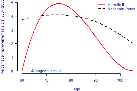
We saw in the previous blog that the Makeham-Perks model had more realistic levels of improvement at the oldest ages compared to, say, the Gompertz model. However, Figure 2 shows that equation (2) for the Hermite family leads to a more sensible pattern of improvements above age 90 that reduce to zero after age 100.
One remaining question is which model produces more accurate improvements between ages 60 and 85? In fact the fits are surprisingly similar: the \(\chi^2\) test statistic against calendar year is 2.95 for the Makeham-Perks model and 2.74 for the Hermite II model. Although the Hermite model is a slightly better fit to time trends overall, neither model comes close to failing the \(\chi^2\) goodness-of-fit test. This is most likely a result of the data being relatively sparse above age 95, which means that the Makeham-Beard model is not being penalised for having such strong improvements for centenarians.
References:
Richards, S. J. (2019) A Hermite-spline model of post-retirement mortality, Scandinavian Actuarial Journal, 2020:2, 110–127.
Richards, S. J. (2020) A value-at-risk approach to mis-estimation risk, Longevitas working paper.
Previous posts
Modelling improvements in experience data - I
In the first of a pair of blogs we will look at how to allow for changes in mortality levels when calibrating models to experience analysis. We start with time-varying extensions of traditional parametric models proposed by actuaries, beginning of course with the Gompertz (1825) model:
\[{\rm Gompertz}: \mu_{x,y} = e^{\alpha+\beta x + \delta(y-2000)}\qquad (1)\]
Piquing interest in improvements
When underwriting a pension scheme for a bulk annuity or longevity swap, the first concern is understanding what mortality levels are, especially differentials amongst sub-groups. The next concern is whether the recent mortality improvements in the pension scheme are in line with the pricing basis; if the scheme has experienced faster improvements, say, then this would be a valuable insight for pricing.
Add new comment