The Poisson assumption under the microscope
If you read almost any paper on modelling mortality you will find the assumption that the number of deaths follows the Poisson distribution. Two well-known papers that use this approach are Brouhns et al (2002) and Cairns et al (2009). The Continuous Mortality Investigation's age-period-cohort-improvements (APCI) model also makes this assumption (Continuous Mortality Investigation, 2016). In this post I put the Poisson assumption under the microscope.
We use data on UK males from the Human Mortality Database (HMD) downloaded on 10th May 2019. We have the number of deaths, \(d_{x,y}\), age \(x\) last birthday in year \(y\) and corresponding mid-year population estimates, the central exposures \(E^c_{x+1/2, y+1/2}\), for ages 0–110+ and for years 1922–2016. Let \(\mu_{x+1/2, y+1/2}\) be the force of mortality at exact age \(x+1/2\) and exact time \(y+1/2\).
An interesting aside is that the death data are exactly the same as that provided by the Office for National Statistics but the exposure data differ significantly. The difference arises from recent changes in the way that the HMD estimates exposures between census dates; the new method adjusts the exposures to take better account of the cohort information found in the relevant birth data.
We assume that \(D_{x,y}\), the random variable corresponding to the observed deaths \(d_{x,y}\), follows the Poisson distribution with mean \(E^c_{x+1/2, y+1/2}\, \mu_{x+1/2, y+1/2}\). We fit a two-dimensional \(P\)-splines model to the data for ages 60–100 and years 1970–2016. We obtain the estimates of the force of mortality, \(\hat\mu_{x+1/2, y+1/2}\); the estimates of expected deaths follow as \(\hat d_{x,y} = E^c_{x+1/2, y+1/2} \hat \mu_{x+1/2,y+1/2}\). Under the Poisson assumption we have
\[\mbox{Var}(D_{x,y}) = E^c_{x+1/2, y+1/2}\, \mu_{x+1/2, y+1/2} \approx E^c_{x+1/2, y+1/2}\, \hat \mu_{x+1/2, y+1/2} = \hat d_{x,y}.\]
Hence, the Pearson residuals
\[z_{x,y} = {d_{x,y} - \hat d_{x,y} \over \sqrt {\hat d_{x,y}}} \sim {\cal N}(0,\,1)\]
approximately. We could also use deviance residuals here. The minimum value of \(\hat d_{x,y}\) is 49.9 so there will be very little difference in the values of the two kinds of residuals; see our book Modelling Mortality with Actuarial Applications (Macdonald et al, 2018, p101-104) for a careful discussion of residuals in the context of mortality modelling.
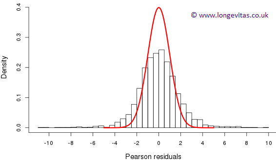
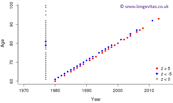
Figure 1 is a histogram of the Pearson residuals with a \({\cal N}(0,\,1)\) distribution overlaid. Evidently, there is far more dispersion here than we would ever reasonably observe from a standard normal distribution. Indeed, the maximum and minimum values of these residuals are 9.6 and \(-10.7\) respectively. Further, there are twenty-three residuals greater than five and twenty-four less than minus five. Figure 2 is a plot of the locations of these large residuals. We see immediately that all of the positive residuals are from the birth cohort of 1920 while all but two of the negative residuals are from the adjacent birth cohort of 1919. The birth cohort of 1920 experienced an excess of deaths; it was a "bad" year to be born. Conversely, 1919 was a "good" year to be born with the cohort experiencing lower deaths than expected. The remaining two negative residuals are from the year 1977 where most of the residuals are negative; 1977 was a "good" year for deaths.
The deaths in the birth cohorts of 1919 and 1920, and the year 1977 are examples of systematic effects; our smooth model doesn't hold in these cells. A similar plot to Figure 2 for residuals with absolute values greater the three shows a more random scatter of large residuals. This is the phenomenon of over-dispersion; there is more variation in the number of deaths than the Poisson distribution allows. The mean and variance of the Poisson distribution are equal. We need to introduce an independent scale parameter without altering the estimates of the underlying mortality surface; this is the so-called dispersion parameter, which we denote \(\phi^2\) (for the Poisson distribution \(\phi^2 = 1\)). This approach is known as the quasi-Poisson model; see Macdonald et al (2018, p203–205) for further details. In our example we found \(\hat\phi^2 = 3.73\). The estimates of \(\mu_{i,j}\) stay exactly the same but their variance is inflated by a factor of 3.73.
Overdispersion is very common for national data of the kind used here, but also for data of insurer portfolios where duplicates are present. Some of the principal reasons include:
- heterogeneity: populations consist of strata with approximately homogeneous mortality; socio-economic group is just one example.
- annual variation: there are "good" years (no flu, mild winters) and "bad" years (flu and/or cold winters) with significantly different mortality, especially at the older ages.
- cohort effects: some cohorts have a "good" mortality while other cohorts are not so lucky.
What are the consequences of staying with the Poisson distribution? Our estimates of mortality and importantly our forecasts of future mortality will be made with greater precision than are justified by the data. Ignoring overdispersion leads to what Moroney (1951) memorably called "delusions of accuracy". Checking the cause of the over-dispersion here allowed us to identify some systematic issues with the data. And since the model forecasts depend on these data, we are reminded always to use models with a critical and questioning mind.
References:
Brouhns, N., Denuit, M. and Vermunt, J.K. (2002). A Poisson log-bilinear approach to the construction of projected lifetables. Insurance: Mathematics and Economics, 31, 373–393.
Cairns, A. J. G., Blake, D., Dowd, K., et al. (2009). A quantitative comparison of stochastic mortality models using data from England and Wales and the United States. North American Actuarial Journal, 13, 1-35.
Continuous Mortality Investigation (2016) CMI Mortality Projections Model consultation - technical paper. Working paper 91.
Macdonald, A. S., Richards, S. J. and Currie, I. D. (2018). Modelling Mortality with Actuarial Applications, Cambridge University Press: Cambridge.
Moroney, F. J. (1951) Facts from Figures, Penguin Press: London.
Add new comment