Longevity trend risk under Solvency II
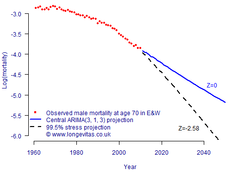
Longevity trend risk is different from most other risks an insurer faces because the risk lies in the long-term trajectory taken by mortality rates. This trend unfolds over many years as an accumulation of small changes, so a natural approach is to calculate reserves using a long-term stress projection from a stochastic model, as shown in Figure 1.
Figure 1. Central projection from a Lee-Carter model, together with the lower 99.5th confidence level derived from multiplying the projection standard error by Z=-2.58 (this being the lower 99.5th point of the N(0,1) distribution).
The stressed-trend approach behind Figure 1 can be used for a variety of models — Table 1 shows the best-estimate and 99.5th percentile stress reserves, together with the implied capital requirements. Table 1 illustrates model risk, namely the tendency for different models to produce different central and stressed estimates, and thus different capital requirements.
Table 1. Central and stressed estimates of present value of continuous annuity payments to a male aged 70. Models of male mortality applied to data from England & Wales, 1961–2010, ages 50–104. Temporary annuities to age 105 are used to avoid distortions caused by extrapolation to higher ages. Discounting is at 3% per annum.
| Model | Central estimate |
99.5% stress scenario |
Capital |
|---|---|---|---|
| Lee-Carter (1992) | 12.20 | 12.96 | 6.28% |
| Cairns-Blake-Dowd (2006) | 11.96 | 12.70 | 6.22% |
| Age-Period-Cohort (APC) | 12.59 | 13.14 | 4.35% |
Table 1 shows the capital requirements for a long-term stress scenario unfolding over the lifetime of the annuitant. However, two useful questions in risk management and reserving are:
- What could happen over the coming year to change the best-estimate projection?
- By how much could the best estimate change based on new information?
Furthermore, the pending Solvency II regulations for insurers and reinsurers in the EU are specifically concerned with the setting of reserves to be adequate in 99.5% of situations which might arise over the coming year. At a high level we could use a stochastic model to simulate the mortality experience of an extra year, and then feed this into an updated model to see how the central projection is affected. This is illustrated in Figure 2, and the process would be repeated many times to generate a probability distribution of how the central projection might change over the same one-year time horizon.
Figure 2. One-year approach to longevity risk. Experience data for 2011 are simulated using an ARIMA(3, 1, 3) model and the Lee-Carter model is refitted each time the 2011 data are simulated. The changes in central projections give an idea of how the best estimate could change over the course of a year based on new data.
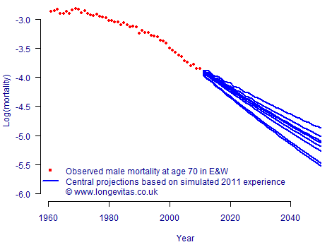
We choose to include both volatility and trend risk in our one-year simulation, but in practice the volatility element dominates over such a short time period. After following the procedure in Figure 2 we have a set of realised values of how life expectancies or annuity values can change based on the addition of a single year’s data. These can then be used to set capital requirements to cover potential changes over a one-year time horizon, as shown in Table 2.
Table 2. Central and 99.5th percentile scenarios for annuity factor for a male life aged 70, using 1,000 simulations of one year's further experience. Models of male mortality applied to data from England & Wales, 1961–2010, ages 50–104. Temporary annuities to age 105 are used to avoid distortions caused by extrapolation to higher ages. Discounting is at 3% per annum.
| Model | Mean | 99.5th percentile |
Capital |
|---|---|---|---|
| Lee-Carter (1992) | 12.22 | 12.83 | 4.99% |
| Cairns-Blake-Dowd (2006) | 11.96 | 12.43 | 3.91% |
| Age-Period-Cohort (APC) | 12.60 | 12.97 | 2.96% |
The mean annuity values in Table 2 are very close to the central estimates in Table 1, but the percentiles are lower. As a result, the capital requirements shown in Table 2 are lower than their equivalents in Table 1. This is partly because the data behind the models in Table 1 end in 2010 and project rates forward to 2011 and beyond. In contrast, the data behind the models in Table 2 end in 2011, so there is one year’s less uncertainty in the projections. As always, model risk is illustrated by the varying capital requirements.
This value-at-risk (VaR) approach can accommodate any stochastic projection model which is parameterized by fitting to data and which is capable of generating sample paths. Models which have arbitrary limits to mortality reduction would not be useful, but most mainstream stochastic projection models fit neatly into this framework. Of course, there is more to longevity risk than this under Solvency II, so the figures in Table 2 would be best regarded as lower bounds.
Value-at-risk in the Projections Toolkit
The value-at-risk for longevity trend risk can be calculated by using the ![]() facility. The user can specify the ages and interest rate (or yield curve) for calculations of life expectancies and annuity factors. The resulting output provides an estimate of the one-year 99.5% capital requirements, either on a value-at-risk basis or a conditional tail expectation (CTE).
facility. The user can specify the ages and interest rate (or yield curve) for calculations of life expectancies and annuity factors. The resulting output provides an estimate of the one-year 99.5% capital requirements, either on a value-at-risk basis or a conditional tail expectation (CTE).
Add new comment